Essay on Consumer’s Equilibrium | Economics

In this essay we will discuss about the effects of changes in income and price on consumer’s equilibrium. 

A consumer is in equilibrium when he maximizes his satisfaction subject to a limited money income and given market prices of goods and services.

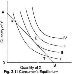
Fig. 3.11 illustrates the consumer’s equilibrium. The budget line is AB and the indifference curves I, II, III and IV are a portion of an individual’s indifference map. Because of the limited money income, the consumer cannot attain a position beyond the budget line. Three of the infinite numbers of attainable bundles on AB are represented by the points R, E and T. Each of these and every other point on the budget line AB are attainable with the consumer’s limited money income.

Suppose the consumer were located at point R. Let the consumer move to combinations of the two commodities just to the left and to the right of R. If he moves to the left he reaches to some lower indifference curve. But moving to the right brings the consumer to a higher indifference curve until he reaches the point E. But moving to the right of E, the consumer would move to a lower indifference curve with its lower level of satisfaction. The consumer would accordingly return to the point E.

Similarly, if a consumer were situated at a point such as T where he can possesses a little of Y and a lot of X. He would very much be interested to substitute Y and X. The substitution enables him to move in the direction of E. The consumer would not stop short of E because each successive substitution of Y for X brings him to a higher indifference curve. Hence the position of maximum satisfaction is attained at E where the consumer is in equilibrium. At the point of equilibrium an indifference curve is just tangent to the budget line.

Let us recall that the slope of the budget line is the negative of the price quantity ratio, the ratio of the price of X to the price of Y. Also recall that the marginal rate of substitution is the negative of the slope of an indifference curve. Hence at point E, the point of consumer equilibrium- or the maximization of satisfaction subject to a limited money income- satisfies the condition that the marginal rate of substitution of X for Y equals the ratio of the price of X to the price of Y.

Algebraically the point of consumer’s equilibrium can be expressed by the condition,

MRS_{x for y} = MU_x/MU_y = P_x/P_y.

Or, equivalently

MU_x/ P_x MU_y/ P_y.

Effects of Changes in Income:

An increase in money income shifts the budget line upward and to the right, and the movement is a parallel shift because nominal prices are assumed to be constant. Changes in consumer’s income lead to changes in his capacity to buy goods and services, other things remaining constant. These changes are depicted by a parallel upward or downward shift in the consumer’s budget line.

Income Consumption Curve (ICC):

As shown in Fig. 3.12, when a consumer’s income increases, his budget line shifts parallel and upward and when his income decreases the budget line shifts downward. As the income changes, a new equilibrium is established and the consumer moves from one equilibrium point to another. Such movements show the rise and fall in the consumption basket. This is termed “income effect”.

Fig.3.12 illustrates the effects of changes in consumer’s income on consumption. Let IC₁ IC₂ IC₃ and IC₄ represent consumer’s indifference map. Given the consumer’s income and prices of goods X and Y, we have his budget line L₁ M₁, the consumer reaches equilibrium at point e₁ on IC₁ consuming Ox₁ units of X and Oy₁ of Y.

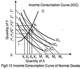
Now let the money income of the consumer increase so that his budget line shifts upward represented by L₂ M₂. The consumer shifts to a new equilibrium e₂ on IC₂ consuming more of both the commodities represented by O x₂ of X and O y₂ of Y. The consumer has clearly gained. Again, if the income of the consumer rises, shifting his budget line to L₃ M₃ establishing a new equilibrium e₃ on IC₃ consuming more of both the commodities X and Y and so on.

As the income of the consumer rises, the budget line as well as the consumer’s equilibrium shifts as well. Thus with each successive upward shift in the budget line, the equilibrium position of the consumer moves upward. The successive equilibrium bundles of goods X and Y at four different level of income are represented by e₁ e₂ e₃ and e₄. The line connecting the successive equilibrium points is called the income- consumption curve.

The curve shows the equilibrium combinations of X and Y purchased at various levels of money income, nominal prices remaining constant throughout. “The Income-consumption curve is a locus of points in the commodity space showing the equilibrium commodity bundles associated with different levels of money income for constant money prices.”

Income Consumption Curve and the Nature of the Commodity:

The effect of changes in income on the consumption of different kinds of commodities is different. It can be positive, negative or even neutral. Infect the nature of a commodity determines whether the effect is positive or negative. The income-effect is positive in case of normal goods and negative in case of inferior goods.

An inferior good is one for which the quantity demanded varies inversely with income- increases in income reduce the quantity demanded and decreases in income increase the quantity demanded of inferior goods. In Fig.3.13, as the income of the consumer increases, the consumption of both the commodities X and Y increases showing positive income effect on both the commodities.

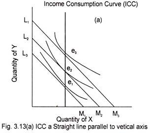
In Fig. 3.13 (a) shows the neutral income effect on a commodity. The ICC is a vertical straight line parallel to the vertical axis showing absence of any income effect on the demand for commodity shown on the horizontal axis (X).

Fig.3.13 (b) and 3.13(c) portray the case of negative income effect. In Fig.3.13 (b) X is an inferior commodity. Its consumption goes on decreasing when consumer’s income increases. Similar is the case in Fig.3.13(c) where the income-effect on Y is negative as Y is considered to be an inferior commodity as its consumption decreases with an increase in the income of the consumer.

Thus the positive or negative income-effect on the consumption of a commodity determines that a commodity is a ‘normal good’ or an ‘inferior good’ If the income- effect is positive, the good is thought to be a ‘normal good’ and if it is negative, the good is considered to be ‘inferior good. Thus depending on the nature of a commodity (normal or inferior), the income consumption curve may take different shapes.

Effects of Changes in Prices:

The impact of a price change on consumer demand can also be ascertained with the help of indifference curve analysis.

When the price of a commodity changes the slope of the budget line of the consumer shifts. The equilibrium of the consumer is also disturbed. A rational consumer, with a view to maximize his satisfaction, tries to adjust his consumption basket. When, the price of a commodity changes, the consumer alters his purchases. A change in the quantity demanded of a commodity due to a change in its price is called the Price-effect.

The price- effect may be defined as the total change in the quantity consumed of a commodity due to a change in its price. Note that it is actually the relative price structure that affects the demand. To investigate the effect of a change in price of one of the commodities, let us retain our two-commodity model, and hold the consumer’s income, his taste and preference and the price of the other commodity (Y) constant.

Fig. 3.14 illustrates the response of a consumer to changes in the price of a commodity shown on the horizontal axis (X) and the resultant change in the bundle of the two goods.

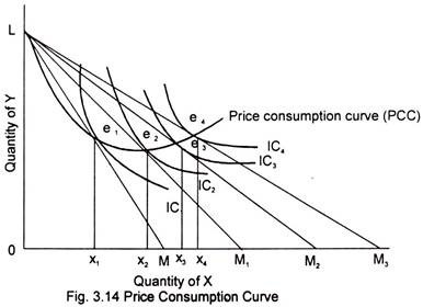
In order to investigate the effects on the consumer’s purchases of changes in the price of one of the commodities let us suppose that the price of one commodity (X) falls, other things remaining constant. This implies that the consumer can buy more of X for his given money income though he can get the same amount of Y as before. We find that a fall in the price of the item on the horizontal axis leads the price line or the budget line flattens out by swinging to the right. With the original price line LM, the consumer reaches equilibrium at point e₁ on IC₁.

When the price of X falls, the new price line is L M₁ and the new equilibrium is attained at e₂ on IC₂ Again when the price of X falls the price line shifts of L M₂ and the new equilibrium is established at e₃. Finally, when the price falls again, the price line is LM₃ and the new equilibrium is at point e₄ on IC₄ If we join all successive points of tangency we get a curve called Price-Consumption Curve or sometimes the offer curve.

Price-Consumption Curve:

The price consumption curve is a locus of points in the commodity space showing the equilibrium commodity bundles resulting from variations in the price ratio, money income remaining constant.

Thus the price-consumption curve (PCC) shows the change in consumption basket due to a change in the price of commodity X. From the Fig.3.14 it can be seen that the quantity of X consumed goes on increasing whereas that of Y first decreases and then increases. The price consumption curve indicates the quantities of X the consumer buys at each price. The curve, therefore, contains the information from which the consumer’s demand curve can be derived.

It may be noted that the price-consumption curve (PCC) characteristically begins at point L, the pivot point of the swinging price line in Fig.3.14, for the reason that, as the price-line approaches the vertical axis, the price of X increases further and further, the consumer finds that he get less and less of X for his money. Eventually, when its price goes high enough, the consumer will be forced out of buying X altogether and he will therefore spend all his money on the remaining commodity Y, i.e. he will buy OL units of Y and no X (point L).

The movement of the consumer along the price-consumption curve due to a fall in the price of a commodity is in reality a resultant of two forces:

(a) Income Effect and

(b) Substitution Effect

A nominal price of a good causes a change in real income, or in the size of the bundle of goods and services a consumer can buy. If the nominal price of one good falls, money income and other nominal prices remaining constant, real income rises because the consumer can now buy more, either of the good whose price declined or the other goods. This change in real income leads to an income effect on quantity demanded.

It should be noted that the shapes of PCC can change if the location of the indifference curves changes as it did in the case of income change. The shape of PCC indicates whether the commodity is price elastic or inelastic or has a unitary price-elasticity. Demand is price elastic if the slope of PCC is negative, price-inelastic if the slope of PCC is positive and unitary elastic if PCC is horizontal

Substitution and Income Effects:

A change in the quantity demanded of a commodity due to a change in its price is called the Price- effect. Price-effect has two components (a) substitution- effect, and (b) income effect. The substitution effect is the change in quantity demanded resulting from a change in relative price after compensating the consumer for the change in real income. In other words, substitution-effect arises due to the consumer’s inherent tendency to substitute cheaper goods for the relative expensive ones.

The income-effect of a change in the price of one commodity is the change in quantity demanded resulting exclusively from a change in real income, at other prices and money income held constant. It arises due to a change in real income caused by a change in the price of the goods. Substitution effect causes a movement along the price-consumption curve that generally has a negative slope. Income effect, on the other hand, causes a movement along the income-consumption curve that has positive slope.

This section will illustrate the methods of measuring the total price effect and splitting the income effect and substitution effect.

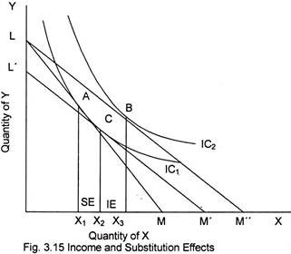
Fig. 3.15 illustrates the substitution effect and the income effect of a decline in price. Let LM be the consumer’s budget line and consumer first be in equilibrium at point A, where IC₁ is tangent to the budget line LM. Now let the price of X fall, the new budget line being LM”. The consumer then moves to a new equilibrium at point B on IC₂. The fall in price causes the consumer to buy more of the commodity X. The additional amount on the horizontal axis is x₁ – x₃ that is identical with the horizontal distance between A and B. The amount AB is the total effect of the change in price.

Now we have to split the price-effect into income and substitution effect. We can find the substitution effect by drawing a line L’M’ parallel to original budget line LM reflecting the new and lower price of X, the dashed line L’M’ represents an imaginary movement of the budget line LM, down to the left. Thus the dashed line stands for an imaginary reduction in income, a reduction of such size as to nullify the gain in real income that comes with the fall in price. The new budget line L’M’ is tangent at point C to IC₁ This point of tangency shows that the consumer would buy x₁ – x₂ more of X independently of the gain in his real income x_{1 –} x₂ represents substitution effect, x₂ – x₃ represents the income effect.