How to Analyse the Internal and External Balances? | BOP | Economics

For analysing the internal and external balances through the synthesis between monetary and fiscal policies, the IS (Investment-Saving) function, the LM (Liquidity preference – Money supply) function and the BOP function (B) are to be derived as below:

Derivation of IS Function:

The investment-saving function (IS) in an open system is determined on the assumption that the real market is in the state of equilibrium. The real market is in a state of equilibrium.

The derivation fiscal of IS function can be made on the basis of the following functional relationships:

In Fig. 25.6, part (i), given (I+X) = f(r), the investment plus exports (I+X) are I₀, I₁ and I₂ corresponding to the rates of interest r₀, r₁ and r₂ respectively. In part (ii), given (S+M) = (I+X) is the equilibrium function. S₀, S₁ and S₂ levels of savings plus imports (S+M) correspond with I₀, I₁ and I₂ amounts of investment plus exports respectively.

In part (iii) of the Fig. given (S+M) = f (Y), the levels of income corresponding to S₀, S₁ and S₂ amounts of saving plus imports are Y₀, Y₁ and Y₂ respectively. In part (iv), given r₀, r₁ and r₂ rates of interest, the corresponding levels of income are Y₀, Y₁ and Y₂ respectively. These income-interest combinations give the IS curve which slopes negatively.

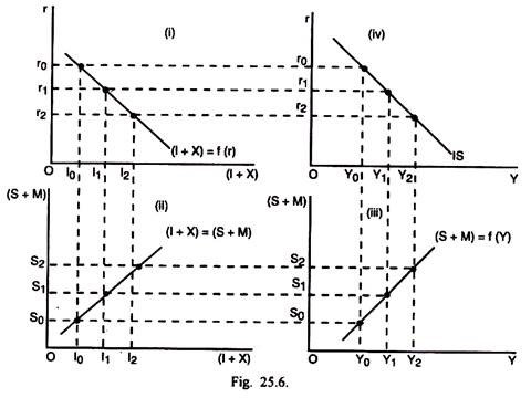
The elasticity of the IS function is determined by the elasticity of I, X, S and M functions. The fiscal policy changes can cause shifts in the IS function. The expansionary fiscal policy involving increase in government expenditure and reduction in taxes can cause a shift in the IS function to the right of its original position and vice-versa.

Derivation of LM Function:

The liquidity preference-supply of money function (LM) is determined on the assumption that money market is in a state of equilibrium.

The derivation of the LM function rests upon the following functional relationships:

L₂ = f(r) (Inverse Function)

L₁ = f /(L₂) (Inverse Function)

L ₁ ⁼ f /(Y) (Direct Function)

Here L₂ stands for idle balances and L₁ for the active balances. The derivation of LM function is shown through Fig. 25.7.

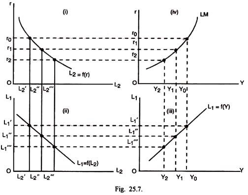
In Fig. 25.7, part (i), given L₂ = f(r), the idle balances corresponding to interest rates r₀ and r₁ and r₂ are L₂‘, L₂” and L₂‘” respectively. In part (ii) of the Fig., given L₁ = f (L₂) the active balances, corresponding to the idle balances L₂‘, L₂” and L₂‘”are respectively L₁‘, L₁“and L₁‘”. In part (iii) of the Fig. given L₁ = f (Y), the levels of income corresponding to active balances L₁‘, L₁“and L₁‘” are Y₀, Y₁ and Y₂ respectively.

Part (iv) of the Fig. shows that r₀, r₁ and r₂ rates of interest correspond with Y₀, Y₁ and Y₂ levels of income respectively. Given these combinations of income and rate of interest, it is possible to derive the LM function which slopes upwards from left to right. The elasticity of LM function depends upon the elasticity of the idle balances curve and the money supply function.

The shifts in the LM function are brought about by the changes in the monetary policy. If an expansionary monetary policy, comprised of increase in money supply and lowering down of the structure of interest rates is adopted, the LM function shifts to the right of its original position. In case of a restrictive monetary policy, this involves reduction in money supply and a rise in the structure of interest rates, the LM function shifts to the left of its original position.

Derivation of the BOP Function (B):

The BOP function is determined on the assumption that the country does not either have a BOP deficit or surplus. It is in a state of BOP equilibrium. It also implies equilibrium in the foreign exchange market.

The derivation of the BOP function (B) can be attempted on the basis of the following functional relationships:

K = f(r) (Direct Function)

K represents the short term capital inflow.

(M-X) = f (K) (Direct Function)

(M-X) signifies the BOP deficit.

(M-X) = f(Y) (Direct Function)

Given these functional relationships, the derivation of the function B can be shown through Fig. 25.8.

In Fig. 25.8, part (i), given K =f(r) the amounts of capital inflow are K₀, K₁ and K₂ at the interest rates r₀, r₁ and r₂ respectively. In part (ii), given (M-X) = f (K), the payments deficits amounts to M₀, M₁ and M₂ corresponding to K₀, K₁ and K₂ capital inflows respectively. Since the BOP function is a 45° line, it signifies that the payments deficit is matched with an equivalent capital inflow so that the system has BOP equilibrium.

In part (iii) of this Fig, given (M-X) =f(Y), the levels of income corresponding to M₀, M₁ and M₂ amounts of BOP deficit are Y₀, Y₁ and Y₂ respectively. Part (iv) of the Fig., shows that Y₀, Y₁ and Y₂ incomes correspond to r₀, r₁ and r₂ rates of interest respectively. Given these combinations of income and rates of interest, the BOP curve B can be drawn. It slopes upwards from left to right.

The elasticity of the BOP function B is determined by the elasticity of capital inflow function [K = f(r)] and the payments deficit function [(M – X) = f (Y)]. Greater is the degree of their elasticity, more elastic is the function B and vice- versa. The shifts in the function B are caused by the variations in exchange rates.

If there is exchange depreciation, the BOP function B will shift to the left of its original position. In the event of exchange appreciation, the BOP function will shift to the right of its original position. If there is a system of fixed exchange rate, the BOP function B will remain unchanged.

We shall discuss below the internal and external balance through monetary-fiscal policy mix under both fixed and flexible exchange systems:

I. Internal and External Balances through Monetary-Fiscal Policy Mix under Fixed Exchange System:

Assuming that a country is having a fixed exchange system and relative capital mobility, the appropriate blend of monetary and fiscal policies can bring about the internal and external balances.

The alternative situations of internal and external disequilibria and their adjustment through the proper monetary and fiscal policy measures have been analysed below:

(i) Internal Unemployment and BOP Deficit:

If a country is faced with internal unemployment and BOP deficit, the internal and external balances can be achieved through the use of expansionary fiscal and restrictive monetary policies under a system of fixed exchange rate. This is explained through Fig. 25.9.

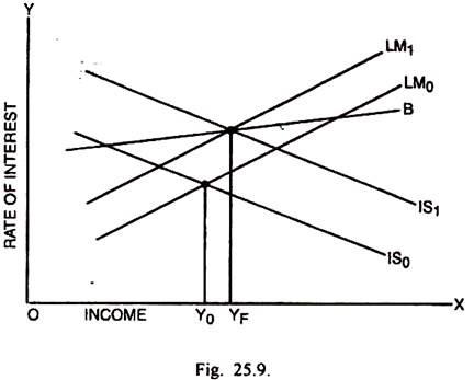
In Fig. 25.9, originally IS₀ and LM₀ are the IS and LM functions respectively and B is the BOP curve. The equilibrium income determined by the intersection of IS₀ and LM₀ is Y₀ which falls short of the full employment income Y_F. Since the intersection takes place below the BOP curve, it signifies the existence of BOP deficit. If the restrictive monetary policy (reduced money and credit and higher interest rate structure) alone is adopted, the LM function shifts to LM₁.

It reduces the BOP deficit but increases the unemployment gap. It is clear from the intersection of IS₀ and LM₁. On the opposite, if the expansionary fiscal policy, comprised of reduction in taxes and increased government spending alone is adopted, the IS function shifts to the right to IS₁. The intersection of IS₁ and LM₀ indicates a reduction in the BOP deficit but the equilibrium income rises beyond the full employment income Y_F.

It means this policy leads to inflationary conditions. If the expansionary fiscal and restrictive monetary policies, given fixed exchange rates and relative capital mobility, are applied simultaneously, the intersection between IS₁ and LM₁ takes place exactly at the full employment vertical Y_F and the BOP curve B. Thus the synthesis of expansionary fiscal and restrictive monetary policies can help achieve the internal and external balances simultaneously.

(ii) Internal Inflation and BOP Deficit:

If there are the conditions of internal inflation along with the BOP deficit, the situation can be tackled and the external and internal balances can be restored through the use of restrictive fiscal policy (high taxes and reduced government spending) and restrictive monetary policy (reduced money supply and high interest rates), given the fixed exchange rates. It can be explained through Fig. 25.10.

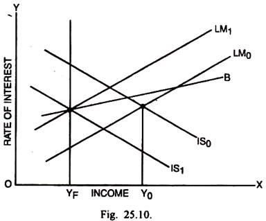
In Fig. 25.10, the intersection of IS₀ and LM₀ originally takes place at the income Y₀ which is more than the full employment income Y_F. Here Y₀Y_F represents the inflationary gap. The equilibrium takes place below the BOP curve B. It signifies the existence of BOP deficit. If the restrictive fiscal policy alone is adopted, the intersection of IS₁ and LM₀ shows that there is an aggravation of BOP deficit. Although inflationary gap has been reduced, yet it has not been fully eliminated.

On the opposite, if the restrictive monetary policy alone is adopted, the intersection of LM₁ and IS₀ shows that BOP deficit has not only been eliminated, there has been, on the contrary, the appearance of BOP surplus as equilibrium now takes place above the BOP curve. At the same time, the restrictive monetary policy, though reduces the inflationary gap, yet fails to remove it completely.

So neither the monetary policy nor the fiscal policy, taken alone, can achieve the internal and external equilibria. If there is a blend of restrictive monetary policy and restrictive fiscal policy, IS₁ and LM₁ intersect each other exactly at the full employment vertical and the BOP curve B and the economy has both internal and external balances.

(iii) Internal Unemployment and BOP Surplus:

When a country is faced with internal unemployment along with the BOP surplus, it is possible to achieve internal and external balances through an admixture of expansionary fiscal and expansionary monetary policies, given a fixed exchange system. It can be explained through Fig. 25.11.

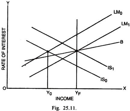
In Fig. 25.11, originally IS₀ and LM₀ determine equilibrium income Y₀ which is short of the full employment income Y_F. It signifies the existence of internal unemployment. The intersection takes place above the BOP curve B. It is indicative of the BOP surplus. In this situation if expansionary fiscal policy is adopted, the IS function shifts to the right to IS₁. The intersection between IS₁ and LM₀ still takes place at the less than full employment level.

At the same time, there is an increase in BOP surplus. So the expansionary fiscal policy neither achieves full employment nor BOP equilibrium. If the expansionary monetary policy alone is adopted, the intersection of LM₁ and IS₀ takes place below the BOP curve.

It means the expansionary monetary policy not only neutralises the BOP surplus but rather creates some payments deficit. At the same time, the unemployment continues to be present though in a smaller magnitude. Thus neither the expansionary monetary policy nor the expansionary fiscal policy alone is equal to the task of achieving both internal and external balances simultaneously.

In case the expansionary monetary and expansionary fiscal policies are adopted together, the intersection of IS₀ and LM₁ takes place exactly at the full employment vertical and also at the BOP curve. So the co-ordinated application of expansionary monetary and fiscal policies, given the fixed exchange system, can help achieve both internal and external balances.

(iv) Internal Inflation and BOP Surplus:

If there are the problems of internal inflation and BOP surplus, these can be properly tackled through the co-ordinated application of restrictive fiscal and expansionary monetary policy, when there is fixed exchange system. The achievement of internal and external balances in such a situation can be explained through Fig. 25.12.

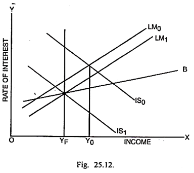
In Fig. 25.12, the original equilibrium income Y₀ is determined by the intersection of IS₁ and LM₀ functions. The income Y₀ is in excess of the full employment income Y_F. There is the existence of inflationary gap Y₀ Y_F in this situation. In addition, the equilibrium occurs above the balance of payments curve B. It signifies the existence of a BOP surplus.

In order to correct the situation, if the restrictive fiscal policy alone is adopted, the intersection of IS₁ and LM₀ takes place at an income even lower than Y_F. It means the restrictive fiscal policy not only removes the inflationary gap but rather creates unemployment. The BOP surplus also continues to exist though in a smaller measure.

In this way, the restrictive fiscal policy is unable to restore the internal and external balances. If the expansionary monetary policy alone is adopted, the intersection of IS₀ and LM₁ shows that there is widening of the inflationary gap. The BOP surplus has no doubt been reduced but it is not completely eliminated. Thus neither the restrictive fiscal policy alone nor the expansionary monetary policy alone can ensure internal and external stability.

If the restrictive fiscal and expansionary monetary policies are applied simultaneously, the intersection of IS₁ and LM₁ takes place exactly at the full employment vertical and at the BOP curve B. Thus a proper synthesis of these policies can lead to the simultaneous achievement of internal and external balances in the conditions of fixed exchange rates.

II. Internal and External Balances through Monetary-Fiscal Policy Mix under Flexible Exchange System:

Under a system of flexible exchange rates with relative capital mobility, the adjustments are facilitated not only by the monetary and fiscal instruments but also through the depreciation or appreciation of exchange rates and consequent movements of capital.

(i) Internal Unemployment and BOP Deficit:

If a country is faced with a large internal unemployment gap and a large BOP deficit, the situation can be tackled through expansionary monetary and expansionary fiscal policies and depreciation of exchange rate. It can be explained through Fig. 25.13.

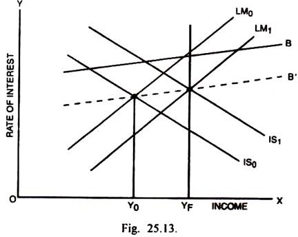
In Fig. 25.13, original equilibrium income is Y₀ which is determined through the intersection between IS₀ LM₀ functions. Y₀Y_f is the large unemployment gap. The equilibrium takes place below the BOP curve B. That indicates the existence also of a large BOP deficit. If the expansionary fiscal policy alone is adopted, the intersection of IS₁ and LM₀ takes place still below the BOP curve B and income is still short of full employment income.

This policy no doubt reduces unemployment gap and BOP deficit but does not completely offset them. If expansionary monetary policy alone is adopted, the intersection of LM₁ and IS₀ takes place still at a less than full employment income and also below the BOP curve. The Fig. shows that the expansionary monetary policy alone somewhat reduces the unemployment gap but there is an aggravation of BOP deficit. So neither the expansionary monetary policy alone nor the expansionary fiscal policy alone can help achieve the internal and external balances.

If the expansionary monetary and fiscal policies are adopted together, IS₁ and LM₁ intersect each other at the full employment vertical. The internal balance has been achieved but the large BOP deficit persists. Under a system of fixed exchange rates, the BOP deficit cannot be neutralised. However, if there is a depreciation of exchange rate, a large inflow of capital can take place from abroad and the BOP deficit can be wiped out.

As a result of exchange depreciation, the BOP curve shifts down from B to B’. Now IS₁, LM₁ and B’ intersect exactly at the full employment vertical. Thus a blend of expansionary fiscal policy, expansionary monetary policy and exchange depreciation can help achieve the internal and external balances.

(ii) Internal Inflation and BOP Deficit:

When a country has to deal with large internal inflationary gap and a large balance of payments deficit, the internal and external stability can be achieved through a proper synthesis of restrictive fiscal policy, restrictive monetary policy and depreciation of exchange rates. It can be explained through Fig 25.14.

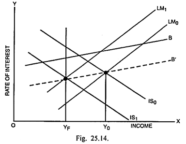
In Fig 25.14, the original equilibrium income is Y₀ which is determined by the intersection IS₀ and LM₀ functions. Since this income is more than the full employment income Y_F, the inflationary gap is of the magnitude Y₀Y_F. The intersection of IS₀ and LM₀ takes place below the BOP curve B. It shows the presence of a BOP deficit.

If restrictive fiscal policy alone is adopted, the intersection of IS₁ and LM₀ still takes place at an income higher than Y_F. The restrictive fiscal policy, no doubt, reduces the inflationary gap but does not completely neutralise it. At the same time, such a policy can result in a further increase in the BOP deficit. In case the restrictive monetary policy alone is adopted, the intersection of LM₁ and IS₀, no doubt reduces the BOP deficit but the inflationary gap is still present, though in a smaller measure.

If the restrictive fiscal and restrictive monetary policies are adopted simultaneously, the intersection of IS₁ and LM₁ takes place at the full employment vertical but the BOP deficit still exists. The exchange depreciation, in this situation, will permit a larger capital inflow from abroad and make way for the BOP equilibrium. As depreciation in exchange rate takes place, the BOP curve shifts down from B to B’.

Now IS₁, LM₁ and B’ intersect at exactly the full employment vertical. It is therefore; clear that the co-ordinate application of restrictive monetary and restrictive fiscal policies along with depreciation of exchange rates can ensure the achievement of both internal and external balances and the situation created by internal inflation and BOP deficit can be tackled effectively.

(iii) Internal Unemployment and BOP Surplus:

If there is large internal unemployment along with BOP surplus, the internal and external stability can be achieved through a proper blend of expansionary monetary policy, expansionary fiscal policy and appreciation of exchange rate. It can be shown through Fig. 25.15.

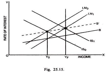
In Fig. 25.15, the IS₀ and LM₀ functions intersect to determine the equilibrium income Y₀ which falls short of the full employment income Y_F. Y₀ Y_F is the unemployment gap. Since the intersection between IS₀ and LM₀ takes place above the BOP curve, it signifies the existence of BOP surplus.

If expansionary monetary policy alone is applied, the intersection of IS₁ and LM₀ results in a reduction in the BOP surplus but it has not been fully offset. Similarly the expansionary monetary policy reduces the unemployment gap but it has not been completely wiped out. On the other hand, if an expansionary fiscal policy is adopted, the intersection of IS₁ and LM₀ leads to a much larger BOP surplus. In this case again the unemployment gap has been reduced but it is not completely eliminated.

If the expansionary monetary and the expansionary fiscal policies are adopted together, the intersection of IS₁ and LM₁ takes place exactly at the full employment vertical but the BOP surplus, given fixed exchange rates, still exists. If the appreciation of exchange rate is permitted, there will be an increased outflow of capital removing the BOP surplus.

So when there is exchange rate appreciation, the BOP curve shifts upto B’. The intersection of IS₁ and LM₁ and B’ takes place exactly at the full employment vertical. Thus the combined application of expansionary monetary and fiscal policies along with an appreciation of exchange rate can effectively tackle the problems of unemployment and BOP surplus and achieve internal and external equilibria.

(iv) Internal Inflation and BOP Surplus:

When there is a large inflationary gap in a country coupled with BOP surplus, the situation can be tackled through an admixture of a restrictive fiscal policy, restrictive monetary policy and an appreciation in exchange rate. This can be shown through Fig. 25.16.

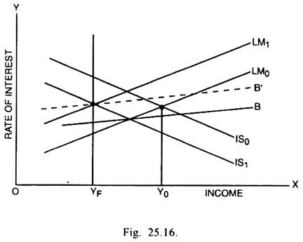
In Fig. 25.16, the original equilibrium income is Y₀ determined by the intersection of IS₀ and LM₀ curves. In this equilibrium position, there is a large inflationary gap Y₀Y_F. If the restrictive fiscal policy alone is adopted, the intersection between IS₁ and LM₀ takes place still at an income higher than Y_F.

There is reduction in inflationary gap but it has not been completely offset. This policy cannot only eliminate the BOP surplus but can also result in some BOP deficit as shown in the Fig. On the contrary, if the restrictive monetary policy alone is adopted, the intersection of LM₁ and IS₀ causes a larger BOP surplus than before. It reduces the inflationary gap but does not completely wipe it out, so either of the two policies taken alone is unequal to the task.

If the restrictive monetary and restrictive fiscal policies are applied together, the intersection of IS₁ and LM₁ no doubt takes place at the full employment vertical but the BOP surplus still persists. If the appreciation of exchange rate is allowed, there will be increased outflow of capital and consequently BOP adjustment can be effected.

The appreciation of exchange rate causes a shift in the BOP curve from B to B’. Thus the combined application of restrictive monetary and restrictive fiscal policies along with an appreciation of exchange rate can deal effectively with internal inflation and BOP surplus and help achieve simultaneously the internal and external balances.