
In this article we will discuss about how to analyse the effect of devaluation upon the balance of payment situation.
In a country having a stable or pegged exchange rate, the removal of balance of payments deficit can be possible through a deliberate policy measure of devaluation. The devaluation of a currency means the deliberate lowering down of the external value of a unit of home currency expressed in terms of gold, SDR’s or a foreign currency by an official edict.
Devaluation is distinct from exchange depreciation in that the latter involves the reduction in the exchange value of home currency on account of the free working of market forces. Devaluation, on the contrary, is the result of deliberate government decision for the achievement of balance of payments equilibrium.
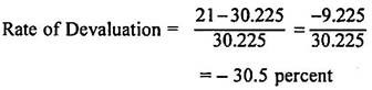
Indian rupee underwent devaluation in September 1949 against pound sterling by 30.5 percent. This measure was a defensive reaction to the devaluation of pound sterling by the United Kingdom. As India’s 75 percent external trade was with Britain, its exports could have suffered grievously. The rate of exchange between rupee and pound sterling prior to devaluation was 1 Re = 30.225 cents and after devaluation it was 1 Re = 21 cents.
ADVERTISEMENTS:
Given these rates of exchange, the rate of devaluation can be computed as below:
Rupee was devalued again in June 1966 by 36.5 percent against pound sterling and the U.S. dollar. This measure was directed to rationalise the exchange rate to increase the competitiveness of Indian exports in foreign markets; to promote import substitution and; to offset the balance of payments deficit.
In July 1991, the Indian rupee was allowed to readjust its exchange rate with the U.S. dollar and pound sterling. This had become necessary on account of sluggish growth of exports and consequent increasing balance of payments deficit.
ADVERTISEMENTS:
This resulted in a decline in the exchange value of rupee between 20.45 percent and 23.07 percent in relation to major world currencies.
As devaluation is undertaken, the home currency becomes cheaper relative to the foreign currency. The foreigners start thinking that the devaluing country has become a cheaper market. Therefore, they direct their demand to that market and the devaluing country finds opportunities to expand its exports. At the same time, the importers of the devaluing country start feeling that the foreign market has become relatively more costly.
This leads to a reduction in the demand for foreign products. The consumers start switching their demand to the home-produced goods. This encourages the substitution of home-produced goods in place of foreign products.
Thus devaluation helps in improving the balance of payments deficit through promoting exports and restricting imports. Even the advanced countries, including the U.S.A., Britain, France, Germany and Japan have resorted to this measure as and when the situation warranted the adoption of it.
ADVERTISEMENTS:
The immediate effects of devaluation are increase in exports and reduction in imports so that the balance of payments deficit can either be reduced or completely eliminated. The achievement of balance of payments equilibrium through devaluation can be explained through Fig. 21.4.
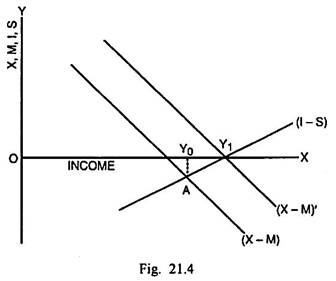
In Fig. 21.4, (X – M) is the net exports or balance of payments function. It varies inversely with income. (I – S) is the net investment function which varies directly with the level of income. Initially given (X – M) and (I – S) function, the equilibrium takes place at the income Y0. In this equilibrium position, there is a balance of payments deficit amounting to AY0.
The devaluation of home currency enlarges exports and reduces imports so that (X – M) shifts upto (X – M)’. Its intersection with (I – S) takes place exactly at the horizontal scale at the income Y1. Since no gap is left between (X – M) and the horizontal scale, the BOP deficit has been completely wiped out.
Regarding devaluation, it should be remembered that the beneficial effects of devaluation are not permanent. These can be available only for a limited time period until the cost-price structure abroad and in the home country does not adjust to the new exchange parity.
The devaluation can bear the desired results and affect payments deficit under the following conditions:
(i) The demand for the exports of devaluing country in the foreign country and the demand for foreign products in the former should be more elastic. If the demand for the exports of devaluing country India in foreign markets is inelastic and the demand for imports from abroad is also inelastic, the devaluation is not likely to remove the BOP deficit. On the contrary, the BOP situation for the devaluing country is likely to get worsened.
(ii) The cost-price structure in the devaluing country should not react in a manner after devaluation that its favourable effects are neutralised. The export prices must be held stable through appropriate governmental restraints upon the activities of speculators and profiteers who are likely to exploit devaluation for raising the prices.
(iii) The devaluation by one country should not be offset by other governments through counter-devaluation measures. Firstly, they should not raise import tariffs on their imports from the devaluing country. Such a policy will neutralise the likely beneficial effects for the devaluing country in the form of larger exports.
ADVERTISEMENTS:
Secondly, the other countries should not readjust their internal cost- price structure at the lower level through export subsidies. Such a policy will make it difficult for the devaluing country to reduce her imports. Thirdly, the foreign countries should not themselves resort to devaluation.
There are two alternative approaches to analyse the effect of devaluation upon the balance of payment situation:
1. The elasticity approach, and
2. The absorption approach.
ADVERTISEMENTS:
The extent by which devaluation can effect an improvement in the payments deficit of a country depends upon the magnitude of the price elasticities of demand for and supply of imports. If the elasticity of demand for the exports of the devaluing country is less than unity (ηx < 1), the devaluation will not reduce the payments deficit of the country.
The balance of payments stringencies, on the opposite, are likely to rise. The devaluation of currency, by say 20 percent, given the elasticity of demand for exports less than unity, will increase the volume of exports by less than 20 percent. This is the positive factor resulting from devaluation.
On the opposite, the price per unit of the export goods will fall by 20%. This is the negative factor which more than off-sets the positive factor. This may result in the negative net effect on the foreign exchange earned by the country. Fig. 21.5 depicts this situation. We assume that there are two countries, India and England. India devalues rupee in terms of pound sterling. We also assume that the elasticity of demand for exports is less than unity.
ADVERTISEMENTS:
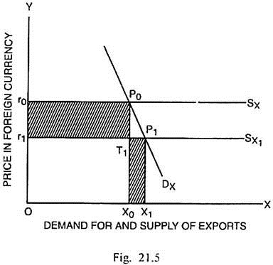
In Fig. 21.5, Dx represents the relatively less elastic demand function of exports and Sx, the perfectly elastic supply function of exports. The foreign exchange rate prior to devaluation of rupee was r0 and the total volume of exports was X0. The total foreign exchange earned was equal to Or0 × OX0 = OX0P0r0. The devaluation results in a lower sterling price of rupee r1.
The supply function of exports shifts down to SX1 and the demand for exports rises to X1. The total foreign exchange receipts in this situation are equivalent to OX1P1r1. Whether the net effect on the foreign exchange receipts, consequent upon devaluation, is positive or negative depends upon whether the area r1T1P0 r0 is less or more than the area X0T1P1X1.
In Fig. 21.5, since r1T1P0r0 is greater than X0T1P1X1, the foreign exchange receipts have decreased. As a consequence, the balance of payments deficit increases. The total volume of exports has gone up but it involves a decline in the foreign exchange receipts. Thus devaluation does not necessarily lead to an improvement in the payment situation.
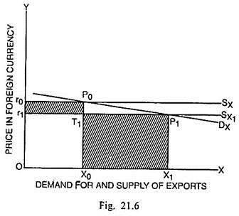
In case the elasticity of demand for exports of the devaluing country is more than unity (ηx > 1), the devaluation will bring about a reduction in the balance of payments deficit. In this situation, a 20 percent devaluation of home currency will raise the volume of exports by more than 20 percent. The improvement in the BOP deficit, in this situation, can be shown through Fig. 21.6.
ADVERTISEMENTS:
In Fig. 21.6, given perfectly elastic supply function of exports Sx and a more elastic demand function of exports Dx, the quantity exported at r0 exchange rate is X0. The receipts from exports are OX0P0r0. After devaluation, at the exchange rate r1, the quantity exported is OX1 and receipts from exports are OX1P1r1.
Since the gain in export receipts X0T1P1X1 is more than loss in receipts r0P0T1r1, there is a net increase in receipts from exports. Therefore, devaluation can improve the balance of payments deficit, when the elasticity of demand for export of the devaluing country is greater than unity (ηx > 1).
On the side of imports, the devaluation will cause the improvement in the balance of payments conditions, if the elasticity of demand for imports is greater than unity (ηm > 1). In this situation, a given percentage increase in the price of imports will result in a more than proportionate fall in the volume of imports leading to a net decline in the payments in exchange of imports. This has been shown through Fig. 21.7.
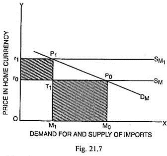
The demand curve for imports (DM) has been taken in Fig. 21.7 as more elastic and the supply curve of imports (SM) as perfectly elastic. Before devaluation, the total volume of imports was M0 and the import price in rupees was r0, so that the total payments on account of imports are equal to OM0P0r0. After devaluation, as the supply curve of imports has shifted to SM1, the amount of imports declines from M0 to M1 and the total import payments are OM1P1r1.
Now since the imports have decreased by M0M1 and the total import payments after devaluation are less than the payments before devaluation, the payments position, consequent upon devaluation of rupees, has improved. The improvement in the payments position can also be measured by the extent by which the shaded area M1T1P0M0 is greater than the shade area r0T1P1r1.
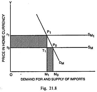
In Fig. 21.8, given a less elastic demand function for imports Dx and perfectly elastic supply function of import SM, the import price in the home currency is r0 and quantity imported is M0. The payments for import amount to O0P0M0. If devaluation takes place, the import price in home currency rises to r1 and the supply function of imports is SM.
Now the quantity imported is M1 and the payment for imports amounts to Or1P1M1. Since the gain in payment for imports r0T1P1r1 is more than reduction in payments M1T1P0M0, there is a net increase in payments for imports after devaluation. It brings home the fact that devaluation worsens the BOP deficit in case the elasticity of demand for imports is less than unity (ηm < 1).
When the supply of exports and that of imports is perfectly inelastic i.e., ex = em = 0 and a country devalues, it will still be possible for the devaluing country to improve her balance of payments, since the price of her exports in terms of domestic currency rises by the full amount of devaluation and the price of her imports in terms of domestic currency fails to rise.
This situation results in the devaluing country receiving larger quantities of imports in exchange for the same quantity of exports or receiving same flow of imports for a lesser quantity of exports. This can be shown through Figs. 21.9 and 21.10.
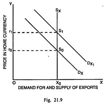
In Fig. 21.9, the demand and supply of imports are measured along the horizontal scale and the price expressed in terms of the home currency is measured along the vertical scale. We assume that India devalues her currency. Since the supply of exports is perfectly inelastic, the price of exports in term of rupees will rise by the full extent of devaluation such that the price rises from r0 to r1.
ADVERTISEMENTS:
In spite of a rise in domestic prices of exports, country’s exports still remain unaffected. This implies that the demand for Indian goods by the foreigners has actually undergone an increase reflected by a shift in the demand function of exports from Dx to DX1. The total payments received by India after devaluation are OX0S1r1 which exceed the receipts before devaluation, i.e., OX0S0r0 by r0S0S1r1. The amount r0S0S1r1 represents the net gain due to devaluation.
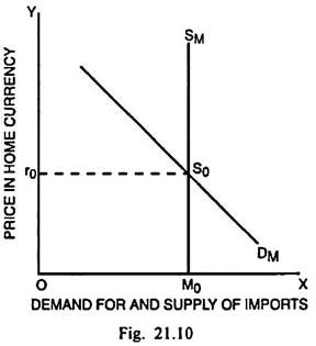
The supply of imports too being perfectly inelastic, as shown in Fig. 21.10, the foreign exporters will have to reduce the prices of their own products in their own currency with the intention of preventing the demand for their goods from declining. The domestic prices of imports in India will, therefore, remain the same.
As a result, the imports from other countries will also remain unchanged at M0 and the total payments which India will have to make in exchange for her imports remain equal to OM0S0r0 even after devaluation.
Marshall-Lerner Conditions:
The above analysis related to the effects of elasticities of demand and supply upon the balance of payments adjustment through devaluation was too general. It is necessary to be more specific in order to predict the effects of devaluation upon the BOP situation. In this connection, Marshall-Lerner conditions can be used. The Marshall-Lerner conditions can specify the situations in which devaluation can successfully improve the balance of trade and payments.
ADVERTISEMENTS:
These conditions are mentioned below:
(i) If the sum of elasticities of demand for exports and imports is greater than unity, devaluation will improve the balance of payments (i.e., reduce deficit).
(ii) If the sum of this elasticity co-efficient is equal to unity, devaluation will leave the balance of trade or payments unchanged.
(iii) If the sum of this elasticity co-efficient is less than unity, devaluation can cause the worsening of the balance of payments (i.e., increase deficit).
These conditions may be illustrated through numerical examples. It is assumed that elasticity of demand for imports (ηm) in a country is 1 and the elasticity of demand for exports (ηx) is also 1 so that the sum of these elasticity co-efficients is greater than unity (ηm + ηx = 2).
If there is 20 percent devaluation, a 20 percent fall in the export price will cause a 20 percent increase in export receipts. On the other hand, a 20 increase in import prices results in 20 percent decrease in imports such that there is no increase in payments on imports. Consequently, there is 20 percent net increase in receipts from exports and BOP deficit will get reduced.
In the second case, it is supposed that ηx = 1/2 and ηm = 1/2 so that the sum of two elasticity co-efficients is unity [ηx + ηm = 1], If there is devaluation at the rate of 20 percent, a 20 percent fall in export prices will cause a 10 percent increase in the exported quantity and the export earnings. On the other hand, a 20 percent rise in import prices causes a reduction in imported quantity by 10 percent. In this case, the payments for imports rise by 10 percent. Thus 10 percent increase in export earnings is fully off-set by 10 percent increase in payments for imports. As a result, the BOP deficit will remain unchanged.
In the third case, it is supposed that % = 1/4 and ηm = 1/2 so that the sum of two elasticity coefficients is less than unity [ηx + ηm = 3/4]. If there is 20 percent devaluation, a 20 percent fall in export prices will cause a 5 percent increase in export earnings.
At the same time, a 20 percent rise in import prices will cause a reduction in quantity imported by only 10 percent. In this situation, the payments for imports increase by 10 percent, so there is a 5 percent net decrease in exchange reserves and the BOP deficit will increase.
The Marshall-Lerner conditions rest upon a fundamental assumption that the supply of export and imports is perfectly elastic. In actual reality, elasticity of supply co-efficients do not have that limiting value. In such situations, nothing can be said offhand i.e., whether the payments position, consequent upon devaluation, will improve or get worsened.
The net change in the balance of payments due to a given change in the rate of foreign exchange has been expressed by L.A. Metzler through the following equation:
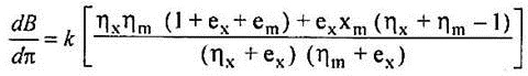
dπ and dB denote the change in foreign exchange rate and a change in the balance of payments respectively.
k denotes the devaluation of currency in terms of percentages.
ηx and ηm refer to the price elasticities of demand for exports and imports respectively.
ex and em refer to price elasticities of supply of exports and imports respectively.
Metzler’s comments about these cases are:
“If exports are produced under constant supply prices, as they are for many manufactured products, both ex and em are infinities, and elasticity on the balance of payments become ηx + ηm = 1. The minimum requirement for stability in this case is, therefore, that the sum of the two demand activities shall exceed unity. At the other extreme, where the supply of exports and imports is completely inelastic, as it is in the short run for certain agricultural products, the elasticity of the balance of payments is always positive and has a value of unity, regardless of the demand elasticities. Under such conditions, devaluation always improves a country’s balance of payments, no matter how elastic the demand for imports may be.”
Between these two extremes, lower the coefficients of elasticities of demand for imports and exports, which are likely to be in the short run, brighter are the chances of improving the balance of payments through devaluation. If the elasticities of supply of exports and imports too are low, the balance of payments can be improved still more quickly.
Criticism of Elasticity Approach:
The elasticity approach as well as the Marshall-Lerner conditions have been criticised on the following main grounds:
(i) Perfectly Elastic Supply of Exports and Imports:
Marshall-Lerner conditions rest upon the assumption that there is perfectly elastic supply of exports and imports. Such an assumption is clearly not realistic. If the devaluing country is not in a position to enlarge the production of exportable commodities, the earnings from exports can be raised. Thus supply inelasticities set a serious limitation upon the success of devaluation in correcting the BOP deficit.
(ii) Neglect of Capital Flows:
The elasticity approaches, in general, and Marshall-Lerner conditions, in particular, are applicable essentially to the commodity trade or the balance of current account. It is only when the devaluation results in sufficient inflow of capital into the devaluing country that the balance of payments deficit is likely to be removed.
In case the devaluation fails to induce sufficient inflow of capital or it causes an increased outflow of capital, the devaluation will worsen the BOP situation even though sum of demand elasticity co-efficients is more than unity. This approach fails to consider the effect of devaluation upon capital movements.
(iii) Partial Elasticities:
The elasticity approach was attacked by S. Alexander on account of the fact that the elasticities used in this approach are the partial elasticities, which excluded everything except relative prices and quantities imported and exported. Such an approach can be valid in case of a single commodity. It fails in case of a multi- commodity trade.
Kindelberger made a modification upon the elasticity approach by taking into account total elasticity co-efficients rather than partial elasticity co-efficients. Alexander refuted this approach and attempted to analyse the effect of devaluation on BOP situation through the alternative ‘absorption’ approach.
(iv) Partial Equilibrium Approach:
The elasticity approach rests upon highly unrealistic assumptions such as full employment of resources, stability of domestic prices and incomes and absence of restrictions upon reallocation of resources. Given these assumptions, the entire analysis is essentially a partial equilibrium analysis. Such an approach is unsuited to consider the feedback effects.
(v) Neglect of Income Distribution:
Devaluation results in reallocation of productive resources from other sectors to the export sector and the import-substitution sector. This leads to a redistribution of income in the economy. The income redistribution effect of devaluation is overlooked by the elasticity approach.
(vi) Off-Setting Effect of Inflation:
The elasticity approach is not likely to measure exactly the effect of devaluation upon the balance of payments. Devaluation causes an expansion in exports and reduction in imports due to decline in the relative prices in the devaluing country compared with foreign countries.
The higher import prices may push up the domestic cost structure in the devaluing country. The expansion of exports raise incomes in the home country. The increased demand for products due to higher incomes may also strengthen the inflationary tendencies.
In addition, the increase in exports may result in domestic shortages and consequent rise in prices. If inflation results from devaluation, it may have the off-setting effects and BOP deficit may not get removed. On the opposite, it is possible that there is worsening of the BOP deficit. The elasticity approach, in such a situation, cannot exactly explain the effect of devaluation on the balance of payments.
(vii) Neglect of Trade Barriers:
The elasticity approach as well as Marshall-Lerner conditions rest upon the assumption that there is absence of tariff and non-tariff restrictions upon trade. Such an assumption is not true in real life.
(viii) Constancy of Price Level:
This approach assumes that there is absence of price changes in the exporting and importing countries. In fact, the price variations, both absolute and relative, continue to take place. In such conditions, the elasticity approach cannot lead to correct conclusion.
(ix) Income Effect Ignored:
As changes result in both exports and imports due to varying elasticity co-efficients, both the trading countries experience the income effects which also influence the BOP surplus or deficit. However, this approach ignores the income effects.
(x) Inadequacy of Elasticity Approach:
This approach alone is not sufficient to determine the success or failure of devaluation in a particular country. Even if the sum of elasticities of demand for exports and imports is more than unity, it does not necessarily mean that the devaluing country will be benefitted. In case the devaluing country has a large volume of external debt, the burden of external debt will increase consequent upon devaluation and the devaluing country will get engulfed by severe financial crisis.
No doubt, there are several theoretical deficiencies in the elasticity approach and Marshall-Lerner conditions. It is relevant to consider the empirical studies related to the estimation of elasticity co-efficients to determine the validity of this approach. Before the World War II, there was a widespread belief that the demand for and supply of foreign exchange were highly elastic. Marshall himself advanced such a view but he could not provide any empirical justification for such a belief.
Some of the empirical studies conducted during 1940’s were rather pessimistic. They suggested that the sums of demand elasticity co-efficients were either less than unity or barely equal to unity. G. Orcutt, however, in his study conducted in 1950, concluded that the regression technique used in the estimation of elasticity co-efficients led to their gross under-estimation.
The subsequent empirical studies made by Harberger (1957), Houthakker and Magee (1969), Stern Francis and Schumacher (1976), Spitaeller (1981) and Artus and Knight (1984), not only attempted to overcome some of the estimation problems raised by Orcutt but supported the view that the elasticity co-efficients were high enough to ensure stability in foreign exchange market not only in the short period but also in the long period.
The study made by Artus and Knight concerning long period indicated that the unweighted average of the sum of export and import price elasticities was 1.92 for the seven largest industrial countries, 2.07 for the smaller industrial countries and 2.0 for all industrial countries. Thus the elasticity approach, in general and Marshall-Lerner conditions in particular, were found to be empirically valid at least in the industrial countries.
The J-Curve Effect:
According to some empirical studies, devaluation leads to the worsening of the balance of trade and payments initially but subsequently it may result in the improvement in the balance of trade and payments. The J-curve depicts the worsening of balance of payments deficit in the short run and improvement of it in the long run due to devaluation. The J-curve has been shown through Fig. 21.11.
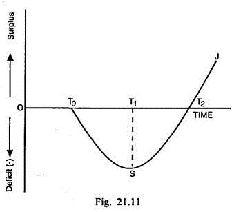
In Fig. 21.11, time is measured along the horizontal scale and the balance of payments surplus and deficit along the vertical scale. Devaluation of home currency takes place in the time T0. Initially it results in the worsening of BOP deficit. The deficit ST1 is maximum in time period T1. Thereafter, deficit starts getting reduced.
There is BOP equilibrium in the time period T2 and later there is surplus in the BOP. Thus the curve depicting the effect of devaluation on BOP follows the shape of letter ‘J’ of the English alphabet and is referred as J-curve.
The J-curve phenomenon occurs on account of a number of reasons. Firstly, according to S.P. Magee, the export contracts are in domestic currency. When devaluation takes place, less foreign exchange is earned from exports. Imports, on the other hand, are invoiced in foreign currency. Devaluation leads to more payments for imports. So long as the old contracts, negotiated before devaluation, are being fulfilled, the balance of trade and payments continues to deteriorate.
The improvement begins to take place, when new contracts after devaluation are negotiated and fulfilled. Secondly, incentive effect of devaluation takes place after some time lag. Until then, the trade balance deteriorates. After the lag expires, there is improvement in the balance of trade and payments.
2. The Absorption Approach:
In the elasticity approach, the devaluation is supposed to affect the BOP situation through price effect. In view of certain theoretical and other deficiencies in that approach, the alternative Absorption Approach was developed by Sydney Alexander.
According to him, the traditional micro approach was deficient as it overlooked the income effect of devaluation. Devaluation can affect domestic consumption, investment and government spending. The absorption approach stresses precisely on that.
This approach can be explained algebraically as follows:
In a state of equilibrium,
Y = C + I + G + (X – M)
This equation can be expressed as:
(X-M) = Y – (C + I + G)
Or B = Y-A
Where B stands for the balance of payments position and A for the sum of consumption, investment and government expenditures. This aggregate of domestic spending (C + I + G) can be called ‘absorption’. C and I are determined by marginal propensity to consume (b) and marginal propensity to invest (a) respectively. G is supposed to be autonomously given. Alexander holds that the sum of b and a is the marginal propensity to absorb (e).
e = b + a
Larger the co-efficient e, lesser are the chances of success of devaluation in wiping out trade deficit and vice-versa.
It is possible to visualise three possibilities in this connection:
(i) If e < 1, there will be improvement in trade balance.
(ii) If e = 1, there will be neither improvement nor worsening of trade balance.
(iii) If e > 1, there will be worsening of the trade balance.
These possibilities can be illustrated through the following numerical examples:
Case I:
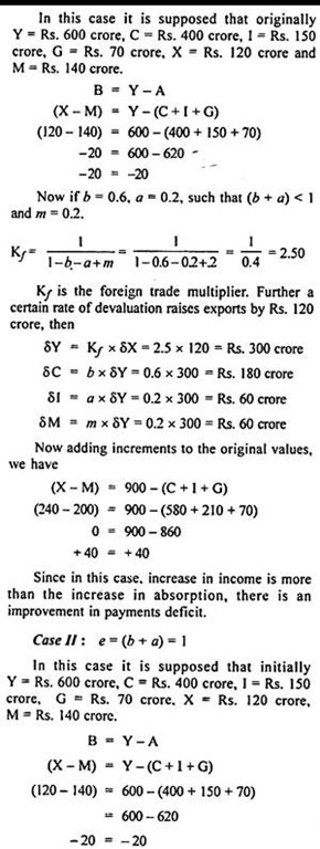
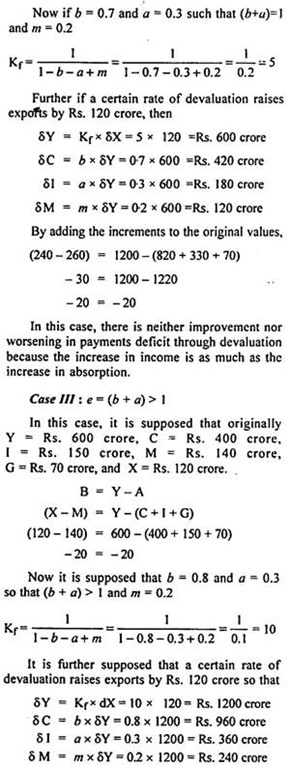
e = (b + a) < 1
In this case it is supposed that originally Y = Rs. 600 crore, C = Rs. 400 crore, I = Rs. 150 crore, G = Rs. 70 crore, X = Rs. 120 crore and M = Rs. 140 crore.
By adding the increments to the original values-
(X-M) = Y – (C + I + G)
(240-380) = 1800-(1360+ 510+ 70)
-140 = 1800-1940
-140 = -140
Thus, in this case, devaluation results in worsening of payments deficit because the absorption has increased by a larger magnitude than the increase in income.
In this approach, the success or failure of devaluation in correcting the BOP deficits in current account is conditioned by the magnitude of the marginal propensity to absorb (e). But apart from e, there are certain other factors which determine the effectiveness of devaluation in correcting BOP deficit.
These factors are as below:
(i) Terms of Trade:
The devaluation may turn the terms of trade against the devaluing country. It tends to reduce real income. The fall in the real income causes a reduction in absorption. If e > 1, the fall in absorption is likely to be more than the decline in real income. Consequently, there can be an improvement in the BOP situation.
(ii) Real Balance Effect:
If devaluation causes a rise in prices, given the nominal stock of money, there will be a fall in the real balances and a rise in interest rates. If people want to maintain an unchanged level of real balances, it is necessary for them to increase savings. It means there should be a fall in absorption. There will also be a fall in real income. Given e > 1, the fall in absorption will be more than the fall in income. In such a situation, devaluation is likely to improve the payments deficit.
(iii) Redistribution of Income:
If devaluation is followed by a redistribution of income from people with high propensity to spend towards those having a low propensity to spend, there is likely to be a reduction in absorption. In this situation, the BOP situation is likely to get improved for the devaluing country.
(iii) Money Illusion:
If people notice a rise in their money incomes and fail to notice a rise in prices subsequent to devaluation, the money illusion is supposed to exist. In such a situation, there may be an increase in absorption and BOP deficit is likely to be reduced.
(v) Expenditure-Reduction Policies:
If the government in a country has followed expenditure- reducing monetary and fiscal policies, the absorption may get reduced and the devaluation can bring about an improvement in the balance of payments deficit.
Criticism of the Absorption Approach:
The absorption approach to devaluation is simple and conceptually neat and straight-forward. It has, however, been criticised on certain grounds. Firstly, this approach was attacked by Fritz Machlup on account of the fact that the whole theorising in it was based upon Keynesian identities and tautologies.
Secondly, even though absorption approach seems to be analytically superior to the elasticity approach, yet a serious flaw in it, that cannot be overlooked is that the propensities to consume, invest and import cannot be exactly determined. Thirdly, this approach restricts itself to the analysis of the impact of devaluation upon domestic absorption. It fails to consider the repercussion effects of increased absorption in the devaluing country upon the foreign country’s national income and balance of payments.
Fourthly, even if it is conceded that devaluation causes a reduction in absorption due to a reduction in consumption spending, yet it does not lead necessarily to redistribution of productive resources from other sectors in the economy to the export and import-substitution sectors. Fifthly, the absorption approach was subjected to severe criticism on account of the fact that it completely over-looked the price effect or the price elasticities of demand for exports and imports.
In view of this criticism from Machlup” and other writers, Alexander attempted to synthesise the elasticity approach with the absorption approach. Tsiang criticised even this synthesis. According to him, that was in fact no synthesis at all. Moreover, Alexander was not original in that exercise. Even before him, that type of synthesis had been attempted by Harberger. Apart from Tsiang and Alexander, these two approaches were synthesised by J.F. Kyle and some other writers.