Relationship between Price Elasticity of Demand and Total Expenditure | Microeconomics

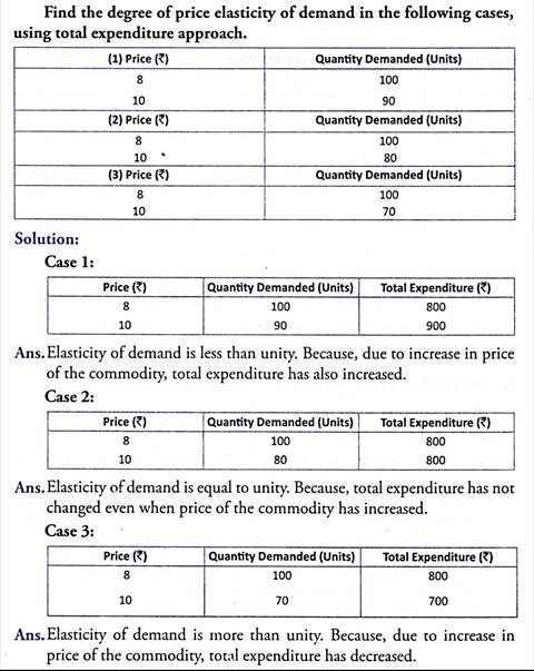
Prof. Marshall works out a relationship between price elasticity of demand and total expenditure. He estimates the degree of price elasticity of demand depending on the change in total expenditure caused by a change in own price of the commodity.

He states three different situations, as under:

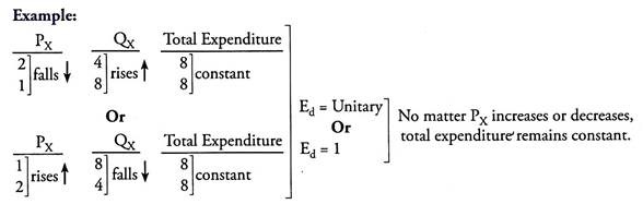
Situation 1 – E_d = Unitary or E_d = 1:

Elasticity of demand is unitary if a rise or a fall in own price of the commodity causes no change in total expenditure on the commodity.

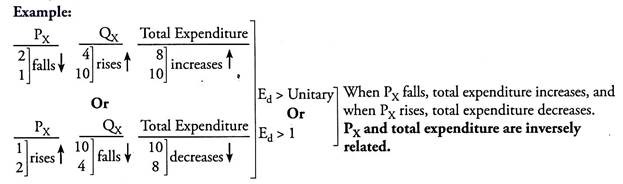
Situation 2 – E_d > Unitary or E_d > 1:

Elasticity of demand is greater than unitary if a fall in own price of the commodity causes a rise in total expenditure, and a rise in own price of the commodity causes a fall in total expenditure on the commodity.

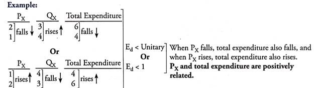
Situation 3 – E_d < Unitary or E_d < 1:

Elasticity of demand is less than unitary if a fall in own price of the commodity causes a fall in total expenditure, and a rise in own price of the commodity causes a rise in total expenditure on the commodity.

Diagrammatic Illustration:

Diagrammatically, the relationship between price elasticity of demand and total expenditure is illustrated through Fig. 3.

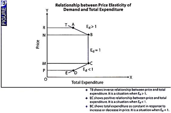
In this figure (Fig. 3), price is shown on Y-axis and total expenditure on X-axis. TE is total expenditure curve. BC part of TE curve represents unitary elastic demand. It shows that when price is OM, total expenditure is MC, as price rises to ON, total expenditure remains constant (= NB = MC). It corresponds to the situation when E_d = 1.

TB part of TE curve corresponds to the situation when E_d > 1. It shows that when price rises from ON to OR, total expenditure falls from NB to RA. Likewise, EC part of TE curve corresponds to the situation when E_d < 1. It shows that when price falls from OM to OP, total expenditure also falls from MC to PD.

Example:

Demand Curves indicating E_d > 1, E_d < 1 and E_d = 1:

We now present diagrammatic illustration of different degrees of elasticities of demand:

Situation 1 – E_d > 1 (Greater than Unitary Elastic Demand):

It is a situation when total expenditure on the commodity is inversely related to change in own price of the commodity.

It implies that:

(i) Total expenditure on the commodity increases when own price of the commodity decreases, and

(ii) Total expenditure on the commodity decreases when own price of the commodity increases.

Fig. 5 illustrates this situation:

Total expenditure = Quantity purchased x Price

When price = OP, quantity demanded = OB,

Total expenditure = OB x OP = area OBTP

When price falls to OP₁, quantity demanded = OC,

Total expenditure = OC x OP₁ = area OCRP₁

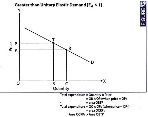
Area OCRP₁ > Area OBTP. Implying that total expenditure increases in response to decrease in price of the commodity.

Hence, elasticity of demand is greater than unity (or E_d > 1).

Situation 2 – E_d < 1 (Less than Unitary Elastic Demand):

It is a situation when total expenditure on the commodity is positively related to change in own price of the commodity.

It implies that:

(i) Total expenditure on the commodity also increases when own price of the commodity increases, and

(ii) Total expenditure on the commodity also decreases when own price of the commodity decreases.

Fig. 6 illustrates this situation:

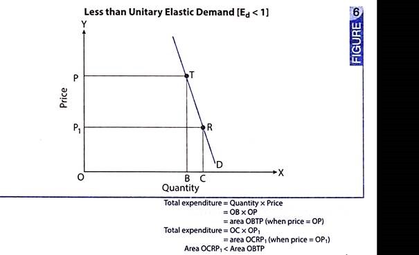
In Fig. 6, when price = OP, quantity demanded = OB, total expenditure is OB x OP = area OBTP. When price reduces to OP₁ and quantity demanded = OC, total expenditure is OC x OP₁ = area OCRP₁. Area OCRP₁ < Area OBTP. Implying that total expenditure is reduced in response to a fall in price of the commodity.

Hence, elasticity of demand is less than unity (or E_d < 1).

Situation 3 – E_d = 1 (Unitary Elastic Demand):

It is a situation when total expenditure on the commodity remains constant, no matter price of the commodity increases or decreases.

Fig. 7 illustrates this situation:

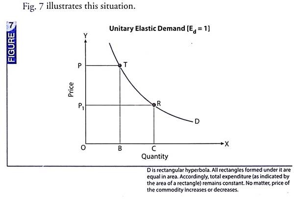
In Fig. 7, demand curve is drawn as a rectangular hyperbola. Its basic property is that all rectangles formed under this curve are equal in area. So that, area OBTP = area OCRP₁. Area OBTP indicates total expenditure when price is OP Area OCRP₁ indicates total expenditure when price is OP₁. Since, area OBTP = area OCRP₁, it implies that total expenditure remains constant even after change in price of the commodity. Hence, elasticity of demand is unity (or E_d = 1).

Three Distinct Situations:

Demand Curve Indicating Same Elasticity of Demand at all its Points:

We have learnt that elasticity of demand is different at different points of a straight line (downward sloping) demand curve. Because, as we move along the demand curve, the ratio between lower segment and upper segment tends to change. However, there are three distinct situations (or three distinct shapes of demand curve) when elasticity of demand is found to be the same at all points.

These are as follows:

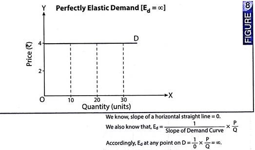
Situation 1 – Perfectly Elastic Demand Curve or a Horizontal Straight Line Demand Curve – E_d=∞ at all Points of the Demand Curve:

A perfectly elastic demand refers to the situation when demand is infinite at the prevailing price. It is a situation when even a slightest rise in price leads to zero demand for the commodity. Fig. 8 illustrates this situation. D is a perfectly elastic demand curve, parallel to X-axis. It shows that if price is slightly increased from Rs. 4, the demand falls to zero. At the prevailing price of Rs. 4, quantity demanded may be 10, 20, 30 or any amount of the commodity. In such a situation, elasticity of demand is infinite (or E_d =∞) at all points of the demand curve.

Situation 2 – Perfectly Inelastic Demand Curve or a Vertical Straight Line Demand Curve – E_d = 0 at all points of the Demand Curve:

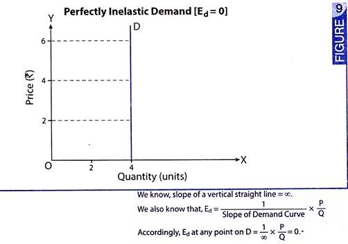
A perfectly inelastic demand refers to a situation when change in price causes no change in the quantity demanded. Even a substantial change in price does not impact quantity demanded. Fig. 9 illustrates this situation. In such situations, demand curve is parallel to Y-axis like D in Fig. 9. When price is Rs. 2, demand is for 4 units. When price rises to Rs. 4 or Rs. 6, quantity demanded remains constant at 4 units. Hence, elasticity of demand is zero (or E_d = 0).

Situation 3 – Rectangular Hyperbola: E_d = 1 at all points of the Demand Curve:

Elasticity of demand is equal to unity (or equal to one) at all points of demand curve when it is a rectangular hyperbola. Rectangular hyperbola is a curve under which all rectangular areas are equal. Because each rectangular area shows total expenditure on the commodity, it implies that total expenditure on the commodity remains constant. No matter price of the commodity increases or decreases. Hence, elasticity of demand is unity (or E_d = 1) at all points of the demand curve as shown in Fig. 10.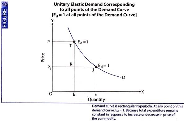Flatter the Curve, Greater the Elasticity:

If two demand curves are shooting from the same point, then flatter the curve, greater the elasticity of demand.

Fig. 11 illustrates this situation

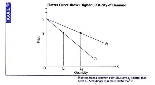
Shooting from the common point S, demand curve d₂ is flatter and therefore, more elastic than demand curve d₁.

This is how it happens:

If price of the commodity falls from OS to OS₁, demand curve d₁ shows a rise in quantity demanded from zero to OL₁, while demand curve d₂ shows a rise in quantity demanded from zero to OL₂. Implying that, for a given change in price, change in quantity is greater corresponding to d₂ than d₁. Hence, d₂ is more elastic than d₁.