
In this article we will discuss about the trade-off between risk and return of investment.
Let us suppose that a person wants to invest his savings in two assets—Treasury bills which are almost risk-free, and a representative group of stocks. He would have to decide how much to invest in each asset. He might, for instance, invest only in Treasury bills, only in stocks, or in some combination of the two.
Let us denote the risk-free return on the Treasury (T.) bill by Rf. Since the return is risk-free, the expected and actual returns are the same. In addition, let the expected return from investing in the stock market be Rm and the actual return be rm. The actual return is risky.
At the time of the investment decision, we know the set of possible outcomes and the probability of each, but we do not know what particular outcome will occur. The risky asset will have a higher expected return than the risk-free asset (Rm > Rf). Otherwise, risk-averse investors would buy only Treasury (T) bills and no stocks.
The Investment Portfolio:
ADVERTISEMENTS:
To determine how much money the investor should put in each asset, let us set the fraction of his savings placed in the stock market equal to b and the fraction used to purchase Treasury bills equal to (1 – b).
The expected return on his total portfolio, Rp, is a weighted average of the expected returns on the two assets:
Rp = bRm + (1-b)Rf (7.6)
Let us suppose, for example, that Rf = 0.4 (or 4%), Rm = .12 (or 12%), and b =1/2. Then
ADVERTISEMENTS:
Rp = 8%. How risky is the portfolio? One measure of its riskiness is the SD of its return, i.e.,
The Investor’s Choice Problem:
We have now to determine how the investor should choose the fraction b. To do so, we have to obtain the equation that would give his risk-return trade-off.
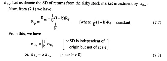
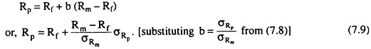
This equation, again, is obtained by rewriting equation (7.1):
Risk and the Budget Line:
Equation (7.9) is a budget line because it describes the trade-off between risk (σRp) and expected return (Rp). Let us note that it is the equation of a straight line. Since Rm, Rf and σRm are positive constants, the slope of the line (Rm – Rf)/ σRm, is also a positive constant as is the intercept Rf.
The equation says that the expected return of the portfolio, Rp, increases as the SD of that return, σRp, increases. We call the slope of this budget line, (Rm – Rf)/ σRm, the price of risk, because it tells us the rate of change of Rp w.r.t. σRp, i.e., how much extra return he requires if he is to accept an additional unit of risk.
For example, he could invest all his funds in stocks (b = 1), earning an expected return Rm, but incurring an SD of σRp = σRm (from 7.8) or, he might invest some fraction of his funds in each type of asset, earning an expected return somewhere between Rf and Rm, and facing an SD (σRp) less than σRm but greater than zero.

Risk and ICs:
Figure 7.6 also shows the solution to the investor’s problem. Three ICs of the investor between risk and return are drawn in the figure. Each curve describes combinations of risk and return that leave the investor equally satisfied. The curves are upward sloping because risk is undesirable. Thus, with a greater amount of risk, it takes a greater expected return to make the investor equally well-off.
Of the three given ICs, IC3 yields the highest level of satisfaction and IC1 the lowest level. For a given amount of risk, the investor earns a higher expected return on IC3 than on IC2, and a higher expected return on IC2 than on IC1.
Therefore, the investor would prefer to be on IC3. This position, however, is not feasible, because IC3 does not take him on to the budget line. The curve IC1 is feasible because the point T1 on IC1 takes him on to his budget line, but the investor can do better.
The investor does the best by choosing a combination of risk and return at the point T2 where an IC, viz., IC2, is tangent to the budget line. The point of tangency between the investor’s budget line and an IC takes him on to the highest possible IC, i.e., the highest possible level of satisfaction, subject to his budget constraint. At that point (here T2) the investor’s return has an expected value R* and at an SD of σ*.