Define Investment in Economics

In this article we will discuss about how investment can be defined in economics.

Introduction to Investment:

Investment plays not only an important role in the static Keynesian model but also in dynamic models of Harrod and Domar who analyse the source of growth. Investment fluctuations as Samuelson and Hicks have pointed out, cause business cycles or income fluctuations. An important aspect of investment is its instability. It is the most volatile component of aggregate effective demand. Net investment fluctuates from negative to positive figures.

With a reasonably stable consumption function, investment fluctuation causes fluctuations in consumption, too. A drop or increase in investment may thus produce only a minor change in the percentage of investment to total output, because it will produce a similar fall or rise in output.

Investment is the accumulation over time by firms of three main types of physical capital goods, viz:

(i) Fixed capital, items such as plant, machinery and buildings, and

(ii) Working capital, which consists of stocks of raw materials, manufactured inputs and final goods await­ing sale, and

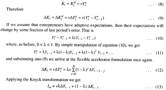
(iii) Residential investment, which includes new houses for purchase or rent.

In private enterprise economies, investment is characterised as gross private domestic investment, that is, residential housing construction and business acquisition of new industrial plants, of machinery and equipment, and of additional inventory. Business fixed investment includes the equipment and structures that businesses buy to use in production. Residential investment includes the new housing that people buy to live in and that landlords buy to rent out.

Inventory investment includes those goods that businesses set aside in storage, including materials and supplies, work in process and finished goods. In this article, we will restrict ourselves to investment in fixed capital, commonly referred to as gross fixed capital formation.

Investment is much smaller in size than consumption. But it is the most volatile component of aggregate effective demand. Moreover, investment in plant, equipment and machinery is very important for the macro economy since such investment determines how much the economy can produce for consumption now and in the future.

Investment is essentially a dynamic proc­ess. It depends on saving which is the difference between disposable income and consumption. The theory of investment is based on the basic premise that consumption has to be sacrificed today in order to enhance production and consumption in the future.

Investment Function:

Economists study investment in order to understand, as clearly as possible, fluctuation in aggre­gate output of goods and services. An investment function is the relation between the acquisition of capital and a set of explanatory variables.

The IS-LM model is based on a simple investment by relating investment (I) to interest rate (i)- I = f(i). This function states that an increase in interest rate reduces investment. We may now look more closely behind this investment function.

We start with the classical theory of investment and then pass on to Keynes’ view on invest­ment. Then we shall explain the theory of induced investment (not originally considered by Keynes) in terms of the acceleration principle. Finally, we conclude with a note on Tobin’s g-theory of investment.

Marginal Productivity of Capital:

According to the classical theory, capital is employed up to the point where its marginal prod­uct is equal to the market rate of interest. The marginal product curve of capital as shown in Fig. 1 is its demand curve. It slopes downward from left to right due to diminishing marginal physical product of capi­tal.

This curve shows that the volume of investment varies inversely with the rate of interest. Since marginal product of capital falls as more and more capital is employed in the production process, additional units of capital will be ac­quired by profit-maximising firms if the rate of interest falls. This means that amount of capital demanded is an inverse function of the rate of interest.

As G. Ackley has put it:

“If we accept the assumption that the marginal productivity of capital declines with increasing employment of capital, both for the firm and for the economy, then the pursuit of maximum profit will lead to a greater employment of capital the lower the rate of interest.”

Expected yields decline because larger output by the firm requires, in the real world of imperfect competition, lower selling prices. This happens even in a purely competitive indus­try when all firms expand their output simultaneously.

However, the interest rate is not the price of capital goods. It is the cost of using financial capital. In fact, the cost of capital and cost of investment are not the same thing. The cost of capital is interest cost which is a flow variable but the cost of investment is the acquisition cost, i.e., the cost of buying a machine or any physical capital which is likely to generate cash flows in future.

Since the interest rate is cost of using (or financing the purchase of) capital goods, business firms make a comparison between the producing of capital goods (in percentage terms) and the rate of interest (expressed in percentage terms) as the relevant price to be paid for using capital goods.

The yield of capital goods is available in the future, over a period whose length depends on the durability of the capital goods. The rupee yield obtainable from a particular capital good in future is the excess of the sale value of goods produced by use of the capital good over all the costs associated with its use including depreciation.

Keynes, however, introduced a new term in 1936, viz., the marginal efficiency of capital or the percentage rate of return or yield which, according to him, is the main determinant of investment in fixed capital. It is expressed as

 

 

where C is the cost of the asset, R₁, R₂, …,R_n are the net rupee yields of the assets (net of depreciation) at the end of years 1, 2, 3,…, n and e is the marginal efficiency of capital which acts as the balancing factor. Keynes defines e as that rate of discount which, when applied to the series of expected rupee yields from the use of the asset, will just reduce their sum to equal the cost of the asset.

According to Keynes, a business firm will compare e with the rate of interest and take decision regarding investment. So long as e exceeds i, new investment in plant equipment and machinery will take place. To put it differently, it pays to invest in a capital good if its cost plus interest on the investment at the going market rate of interest, is less than the rupee yield expected from the asset are its entire economic life.

But due to diminishing marginal efficiency of capital, it will sooner or later be equal to i, at which point the firm will stop. At this stage, the firm’s stock of capital will be optimum. By adding up the demands of capital of all firms we arrive at the aggregate investment demand schedule—or the social investment demand schedule.

In general, more capital-intensive methods produce more output at the same cost than less capital-intensive methods, or they produce the same output at lower cost. And the more capital- intensive methods are the more profitable the lower the interest rate.

As Ackley has put it:

“Additional use of capital, by more capital-intensive methods, adds to output (or reduces its unit cost, exclusive of interest), but the added product (or cost reduction) is of finite magnitude, and decreases as more and more capital is used.”

This means that, ceteris paribus, the lower the rate of interest the higher will be the demand for capital (and the more capital-intensive will be the structure of production). According to Keynes, marginal efficiency of capital varies directly with R and inversely with C. This can be seen from equation (1).

If marginal efficiency of capital remains constant, more investment will take place if / falls. Alternatively, if i remains constant, more investment will take place if marginal efficiency of capital rises. In other words, investment, as Keynes suggested, varies directly with the marginal efficiency of capital and inversely with i.

From the Theory of Capital to the Theory of Investment:

The theory of capital is often wrongly equated with the theory of investment. The two, are different simply because capital is a stock variable, having no time dimension, but investment is a flow variable which is related to a certain period of time.

The theory of capital explains how the optimum stock of capital employed by the firm depends upon the relationship between the cost of assets, their expected yields, and the interest rate. This follows from the assumption of rational — i.e., profit-maximising — behaviour.

In general, lower the cost of acquiring capital goods or the rate of interest at which money is borrowed to buy capital goods, the higher will be the volume of investment of a firm. Those firms which can acquire capital goods at lower prices than other firms or can obtain loans at lower rates of interest than other firms will invest more in income-earning assets like plant, equipment, machinery and other durable (capital) goods than those firms who do not have the opportunity of an advantageous purchase of capital goods or borrowing at low rates of interest.

However, the above hypothesis is true only for firms which are in equilibrium with reference to their use of capital—i.e., to firms whose capital structure has been adjusted to the going rate of interest, cost of capital goods, and expected yields. But this hypothesis is directly relevant to the theory of investment. The reason is that investment occurs when firms are in disequilibrium with reference to their capital structure, i.e., when their capital stock is less or greater than the optimum levels.

In other words, investment occurs when a firm is trying to adjust its actual stock of capital to the desired level. So there are two problems associated with investment theory. The first problem is to explain the optimum (equilibrium) stock of capital for a firm and an economy. The second problem is to explain at what rate investment occurs when the capital stock is not at its optimum. So what we need is a theory relating first to the size of the stock, i.e., capital, and second to the size of the flow, i.e., investment—by which the stock grows or shrinks.

The theory of investment, like that of consumption, can be studied at two levels—at the level of an individual firm, i.e., at the micro-level and at the level of the whole economy, i.e., at the macro-level. At the micro-level the transition from the theory of capital to the theory of investment is a straight-forward exercise. But the development of the theory of investment from the theory of capital at a macro-level is a complex exercise.

If a firm’s actual stock of capital is less than its desired (optimum) level at the existing rate of interest, purchase prices of capital goods, and expected yields and the needed capital goods are readily available in the market (i.e., if capital goods are not produced according to buyers’ specifications or if there is no delivery lag in the capital goods supplying industry), then investment can take place fairly rapidly.

A company will be able to instantaneously adjust its actual stock of capital to the desired level. But this does not normally happen in reality. In most cases, the capital goods- supplying industry is characterised by delivery lags because most capital goods are not readily available but are made to order, i.e., according to the buyers’ specifications.

In such cases, the rate of investment will be determined by the production period of the particular capital goods. This means that the rate of investment is determined by the speed with which capital goods are produced. This factor is not taken into account by the theory of capital.

If a firm’s actual stock of fixed capital (such as machines) exceeds its optimum stock, there will be an act of negative investment, the rate of which will be determined by the rate of wearing out or obsolescence of the particular capital goods. If a firm’s actual inventory exceeds its derived level, the rate of disinvestment will be determined by the rate of sale (in case of finished goods inventory) or by the rate of use in production (in case of raw materials inven­tory). These considerations are outside the scope of study of capital theory.

Capacity Limits of the Capital Goods Industry:

No doubt, the production of future goods is relevant to a single investment. But for the economy as a whole the limit on the rate of investment is set by the productive capacity of the capital goods industry. It is because the optimum stock of capital must always either exceed, fall short of, or just equal the actual stock.

If the optimum exceeds the actual, firms must be desirous of acquiring new capital goods. As a result, the capital goods industry, trying to fill its orders, will be operating at capacity. But unless the optimum stock of capital grows as fast or faster than the actual stock accumu­lates through investment, the actual stock must gradually ‘catch up’ with the optimum. If, then, the optimum stock just equals the actual, net investment would fall to zero. Capital goods would be replaced as soon as they wore out, but no new (net) investment would be made.

If, however, the optimum stock fell short of the actual stock gross investment would be zero, in which case, net investment would be negative at a rate being determined by the rate of depre­ciation. Again, unless the optimum stock were to fall as fast as the actual, a point of equality should eventually be reached, and the rate of net investment should move from negative to zero.

In equilibrium, when the capital stock is fully adjusted to its optimum level, net investment is zero. In spite of this, replacement investment, equal to depreciation, would maintain a certain level of activity in the capital goods producing industries.

Role of Cost of Capital Goods to Determine Volume of Investment:

In reality, the capacity to produce capital goods does not remain fixed as has been assumed so far. Modern economists think of a flexible limit to output of capital goods. But more capital goods can be supplied only at higher prices due to increasing marginal cost of production. This means that the supply curve of capital goods is upward sloping, in which case there is no such thing as ‘capacity’ output of capital goods.

This, in its turn, implies that the cost of capital goods depends on the rate of production of such goods. We may now examine what happens to the rate of investment if the optimum stock of capital exceeds the actual stock, the rate of interest remaining the same.

It has to be noted at this stage of our analysis that one key element in the determination of the optimum stock of capital is the cost of capital goods. A single firm can take this as given. But for the economy as a whole this cost level is variable, and depends on the total rate of investment. In other words, the cost of capital is assumed to vary with the decisions made by all firms taken together.

The ambiguity involved in the concept of the optimum stock of capital can be removed by defining the demand curve for capital (which shows the optimum stock at each rate of interest) in terms of that level of cost of capital goods which would prevail if investment were at a net rate of zero.

In part (a) of Fig. 2 the optimum stock of capital is shown by Keynes’ marginal efficiency of capital (MEC) curve. Each point of the curve indicates not only a given expecta­tion of yields, but also a cost of capital goods associated with the production of capital goods at a rate corresponding to zero net investment. In part (c) we show the upward sloping supply curve of capital goods (S). The cost of capital goods assumed in defining the MEC curve in part (a) is the level of x of part (c).

If, in part (a), the rate of interest is given at i₀, and the existing stock of capital is K₀, then there is a gap between the actual stock and the optimum stock K. This makes new investment profitable, and at a rate shown by part (b) in Fig. 2. The curve MEI (marginal efficiency of investment) begins at level e_i, for this the level of yield from capital goods when the actual stock is K₀ in part (a) and when the cost of production of capital goods is at level x.

The MEI, however, declines as the rate of investment rises, because higher investment rates will raise the cost of production of capital goods. In fact, the MEI of part (b) falls at the same (percentage) rate as the cost (supply price) of capital goods rises in part (c). In this case, investment occurs at the rate of I₀ at which the cost of capital goods is bid up to the desired level. Beyond that level a further increase in the rate of investment would reduce the percentage yield from capital goods below the rate of interest; thus in this case, I₀ is the short-run equilibrium rate of investment.

But, in the long run, investment, at any rate above zero, causes the actual capital stock K₀ to increase. This increase causes the whole MEI schedule to shift downward. For instance, when the capital stock has grown to K_m, the MEI schedule will have shifted downward to the broken line MEV as shown in part (b), leading to a lower rate of investment, i_m. This means that the further growth of K proceeds more slowly toward K.

The theory developed so far is the substance of Keynes’ theory of investment. Keynes, however, defined his investment theory in a confusing way by calling the ‘marginal efficiency of capital schedule’. This showed the amount of investment which would occur at each possi­ble rate of interest.

According to Keynes, it declines for two reasons:

(i) The larger the stock of capital, the lower the expected return from the use of capital assets; and

(ii) The greater the rate of investment, the higher the cost of assets. Investment is carried to the point at which the MEC equated i. In Keynes’ view, the second reason for declining MEC is important in the short run and the first in the long run.

Unfortunately, Keynes’ analysis leads to confusion. He failed to separate the factors relating to the size of the stock of capital with those relating to the rate of investment. This point was first clarified by A. P. Lerner and then by K. Boulding who brought into focus the difference between MEC and MEI.

Acceleration Theories of Investment:

Keynes’ theory of investment is applicable to fixed assets. But A. Aftalian and J. M. Clark developed a new theory of investment, called acceleration theory, which was refined, modified and extended by modern economists in several directions.

This theory is mainly applicable to inventory investment because inventories are normally proportional to sales. But some econo­mists wrongly apply the acceleration theory in case of two other types of business investment also, viz., fixed asset investment and housing investment.

In both classical and Keynesian theories three variables affect investment decisions, viz., the rate of interest, the cost of capital goods and the expected yields from the use of capital goods. An alternative theory, known as the accelerator theory of investment, suggests that the most important factor determining the size of the optimum stock of capital of a firm is the level of demand for its product.

The accelerator principle states that since there is a basic productive relationship between the stock of capital and the flow of output of consumer goods, a rise in consumption expenditures will bring about a more than proportionate rise in investment in fixed capital, and a fall in the rate of increase of consumption expenditures is enough to bring about an absolute fall in net and possibly gross investment. As early as in 1909, Albert Aftalian observed that fluctuations in consumption would lead to magnified fluctuations in investment.

His argument may be interpreted as follows:

Denoting consumption by C, gross investment by I, and capital stock by K, he supposed that replacement investment was a small proportion of the capital stock and that output of consumer goods C required capital in the proportion K = δC; gross investment is then I = δK+ ∆K = α (δC + ∆C).

He observed that, starting from constant consumption and assuming a depreciation rate of δ =1/10, α/0 per cent increase in consumption would lead to a doubling of gross invest­ment; that is, if gross investment is initially equal to replacement, the proportionate rise in gross investment due to an increase in consumption is

 

 

Thus, a slight expansion of the consumption goods industries will result in a much greater expansion of the capital goods industries. However, in 1917, it was J. M. Clark who was the first to formulate, the accelerator principle explicitly as a relationship between derived demand for new capital goods and the rate of change of consumption- “The demand for maintenance and replacement of existing capital varies with the amount of the demand for finished products, while the demand for new construction or enlargement of stocks depends upon whether or not the sales of the finished product are growing.” He argued that a slackening in the rate of increase of consumption may bring about a fall in gross investment.

The accelerator theory or the acceleration principle is based on the assumption that there exists for each good some fixed proportion between the rate of production of that good and the stock of capital needed for its production. Each machine can produce certain (fixed) units of output. So, to produce more output, more machines are to be installed. So the necessary stock of capital (in physical terms) depends on the level of final output.

This supply means that any change in the level of final output will call for a change in the stock of capital in an amount α times the change in output, where α is the additional capital needed to produce one extra unit of output. That is, investment (I) equal α ∆Q.

If I = ∆K = α∆ Q, I will be zero when ∆Q is zero, when national output or income is constant. But if income changes, by a positive or negative amount, investment (disinvestment) will occur, at a rate which is small or large—depending on whether the change of income is small or large.

Implication:

The acceleration principle essentially illustrates a disequilibrium situation. It shows that the economy’s capital market is always in a state of disequilibrium, because most, if not all, firms are constantly trying to adjust their capital stock to the desired level. In other words, there is no role for the allocation principle in equilibrium.

The point may be proved as follows:

The equilibrium condition of national income in a three-sector economy is

Y_t = C_t + I_t + G_t … (1)

Suppose the consumption function is lagged by one year

C_t = a + bY_t-1 … (2)

and the investment function is

I_t = I_a + I_p = I_a + α (C_t – C_t-1) … (3)

where I_t is total investment, I_a is autonomous investment and l_p is induced private investment and I_p is proportional to absolute change in consumption spending and a is the proportionality factor. Here we are doing a simple exercise—known as period analysis, in which the period is defined as having the length of the consumption lag. Equation (3) asserts that investment will occur in this period at a level sufficient to supply the extra capital goods needed to produce the additional output of consumer goods which has occurred since last period, plus a constant, viz., autonomous investment (I_a).

Substituting from (2) into (3) and then from both into (1) give us the following results:

 

 

 

 

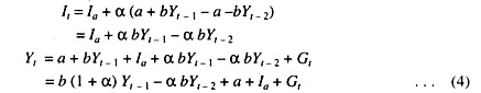
Equation (4) tells us that current year’s income depends on the incomes of the last two years plus the current level of government expenditures. In case the equilibrium income level associ­ated with any given values of a, b, I_a and α, and any given level, G₀ of government expendi­tures can be found by setting

 

 

 

 

This is the usual multiplier formula in a three-sector closed economy, in which income equals the expenditures which are independent of income, times the multiplier. It is interest­ing to note that the acceleration coefficient, a, drops out of the expression for equilibrium income.

The reason is easy to find out: investment occurs as a result of the acceleration principle only when income is changing; equilibrium means stable income, therefore, the acceleration principle plays no role in the equilibrium situation (where there is no change). This proves that the acceleration principle works only when the economy’s capital market is in disequilibrium.

Implication:

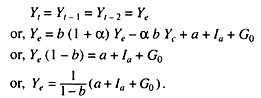
The second major implication of the acceleration principle is that the in­vestment called for by the accelerator be completed in the same period as that in which the additional consumer goods output occurs which required the investment. But in reality this does not happen. The construction and installation of plant and equipment requires some time. So there is no immediate increase in investment following an increase in the demand for consumer goods. This is why modern economists have referred to the lagged accelerator effect, making it

I_t = I_a + α (C_t – C_t-1) … (3)’

Now the levels of b and a are consistent with the achievement of the equilibrium position. Modern economists have also made the accelerator apply to changes in total output, not merely in the output of consumer goods. For added output of capital or government goods should, by the same logic, also require added investment (unless we assume that the capital goods industry always has excess capacity).

Thus we have:

It is likewise possible to work with an un-lagged rather than a lagged consumption function.

Defects:

The main defect of the accelerator relationship is that it is given too fixed and rigid a form. Moreover, with a lag in consumption, customers’ order (if it involves added business) can­not be filled until new machines are built, installed and operating.

The accelerator principle suggests that there is full capacity utilisation in the industries producing consumer goods. If there is idle capacity in such industries, extra output can be produced without making additional investment in plant, equipment and machinery.

Even if all regular equipment is in use, a rise in demand for consumer goods can be met, at least for a short period, by drawing down inventories, by working overtime, by extra shifts and by pressing into service standby equipment. But it is not possible to reduce inventories below zero, and production through overtime, extra shifts, and standby equipment is very costly.

If the increase in demand for consumer goods (and the consequent rise in business) is expected to endure for a long period to make it worthwhile new equipment will be ordered. On the other hand, if the rise in consumption demand is expected to be of a temporary nature, the added demand will be met by running down inventories, by working extra hours, by utilizing idle machines or even by raising the price of the product. Only if the rise in demand is expected to be of a permanent nature will the pursuit of maximum profit lead the entrepreneur to install new machines and equipment.

Another defect of the acceleration principle is that its value does not remain constant over time. Instead, it is affected by calculations of future profitability over the entire economic life of the new machines. The fixed accelerator calls for the entrepreneur to assume, in these calcu­lations, that future demand (in physical terms) is always precisely equal.

Instead, we know that entrepreneurs may expect future levels of demand to rise (fall) above (below) the current level. Such calculators also involve expectations as to future price levels, as well as the cost level of assets, their availability and the interest rate.

The neglected cost and availability of assets is perhaps the most serious defect of the accel­erator theory. The theory ignores any limit on the rate of production of capital goods. The theory suggests that irrespective of the rate of increase in the demand for final products, the necessary capital goods can be immediately produced, in which case the optimum stock and actual stock always coincide.

Comparison with Keynes’ Theory of Investment:

In Keynes’ theory, there is a difference between a capital theory (relating to the optimum stock of capital) and an investment theory (describing how the optimum stock is approached). The acceleration principle uses a single theory for both the jobs. If, instead, we use the basic idea of the accelerator—that the optimum stock of capital depends on output—only as the theory of capital, we have to note an important point.

When the optimum stock and the actual stock diverge, investment will occur, at a rate governed by supply conditions in the capital goods industry (if investment is positive), and at a rate governed by the speed of wearing-out of existing capital goods (if investment is negative).

Further Notes on the Accelerator Principle:

The accelerator principle is based on the implicit assumption that business firms must continu­ally evaluate the size of their factories and the numbers of their machines. The accelerator hypothesis states that the level of net investment depends on the change in expected output. The hypothesis relies on the simple idea that firms attempt to maintain a fixed relation between their stock of capital (plants and equipment) and their expected sales.

Estimating Expected Sales:

The first basic ingredient in a business firm’s decision about plant investment is an educated guess about the likely level of sales. A firm is assumed to revise the estimate of expected sales (Y_t^e) from the estimate of the previous year (Y ^e _t-1) by some proportion, j, of any difference between last year’s actual sales outcome (Y_t-1) and what was expected

Y^e_t = Y_t-1 + Y^e_t-1 – jY^e_t-1 = Y_t-1 + (1 – j) Y^e_t-1 … (1)

Thus, estimate of expected sales is based on the so-called adaptive or error-learning method.

Dependence of Investment on Output Change:

The next step in the accelerator hypothesis is the assumption that the stock of capital – that is, plant and equipment—that a firm desires (K*) is a multiple of its expected sales:

K* = v * Y_e … (2)

The multiple v * relates desired capital to expected sales. In calculating v * firms pay attention to the interest rate and tax rates. Their chosen value of the multiple v * reflects all available knowledge about government policies and the likely profitability of investment.

Net investment (I_n) is the change in the capital stock (∆K) that occurs in each period:

I_n = ∆ K = K_t – K_t-1 … (3)

We assume that a company always manages to acquire new capital quickly enough to keep its actual capital stock (K) equal to its desired level (K *) in each period:

I_n = K_t – K_t-1 = K*_t -K*_t-1 … (4)

In other words, net investment (I_n) is always equal to the change in the desired capital stock in each period, which is a multiple of the change in expected sales:

I_n = K*_t -K*_t-1

= v*(Y_e – Y_t-1) = v* ∆Y_e … (5)

The accelerator hypothesis says that the level of net investment (I_n) depends on the change in expected output (∆Y_e). When there is an acceleration in business and expected output in­creases, net investment is positive, but when business decelerates and expected output stops increasing, net investment actually falls. And, if expected output were ever to decline, net investment would become negative.

Adding Replacement Investment:

Total business spending on plant and equipment includes not only net investment—purchases that raise the capital stock—but also replacement purchases that simply replace old decaying plant and equipment or plant and equipment that has become obsolete.

The total or gross investment (I) is the sum of net investment (I_n) and replacement invest­ment (D).

The Simple Accelerator:

The relation between gross investment (I) and GNP (Y) for the economy as a whole, according to the accelerator hypothesis, is the same as that for an individual firm. In the special case, when expected sales are always set equal exactly to the last period’s actual sales, Y^e = Y_t-1 so that ∆Y^e = Y_t-1. This allows us to rewrite equation (5) as

I_m = v*∆Y_t-1 … (6)

Net investment (I_nt) equals a multiple of last period’s change in sales or output (∆y_t-1). Equation (6) is the simplest form of the accelerator theory and was invented when J. M. Clark, in 1917, noticed a regular relationship between the level of wagon production and the previous change in railroad traffic.

Equation (6) aptly summarizes the inherent instability of the private economy. Any random event—an export boom, an irregularity in the timing of Government spending, or an upward revision of consumer estimates of permanent income—can change the growth of real sales and alter the level of net investment in the same direction.

Defects of the Simple Accelerator:

The simple accelerator theory of equation (6) depends on several restrictive and unrealistic assumptions.

A more realistic version of the theory, called the flexible accelerator, can be developed by relaxing some of these restrictive assumptions:

1. The simple accelerator assumes that this period’s expected output was always set equal to the last period’s actual output. But the error-learning or adaptive hypothesis states that, in gen­eral, only a fraction of expected output is based on the last period’s output, and the rest carries over whatever was expected in the last period.

2. The simple accelerator assumes that the desired capital stock (K *) is set equal to a con­stant (v *) times expected output (Y^e). But, in reality, there is a considerable variation in the desired capital-output ratio (v *), depending on the cost of borrowing, the taxation of capital, and other factors.

3. The simple accelerator also assumes that firms can instantly put in place any desired amount of investment in plant and equipment needed to make actual capital of this period (K) equal to desired capital (K *). Actually, it takes a long time to construct some types of capital, such as office buildings, steel plants and power plants.

Moreover, installing too much new investment at one time would be excessively costly because firms supplying capital goods might raise their prices and the installation activity might disrupt the flow of production.

Thus, net investment in the real world does not always close the whole gap between the desired capital and the last year’s capital stock, but only a fraction of it. The flexible accelerator is the theory that the desired ratio of capital to expected output may be affected by the user cost of capital.

For empirical purposes, the flexible accelerator is found to perform better. We may now discuss this version of the accelerate theory in detail.

The Flexible Accelerator:

The flexible accelerator model, developed by Richard Goodwin in 1948 and refined and modi­fied by L.M. Koyek in 1954, says that investment is still determined by the demand for output, but the feedback from changes in production are more complex and, often, indirect.

There are two potential reasons for this: either the firm faces lags in the delivery of capital goods, or firms are slow to change their expectations of future demand for their products. These two points explain why the flexible accelerator is more complex in its operation than the naive (simple) accelerator.

This point may now be explained in detail:

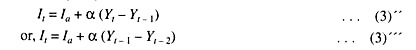
Incomplete Adjustment and Delivery Lags:

In reality, most firms face delivery lags. Capi­tal goods are not supplied as soon as they are ordered. This means that although the firm may be desirous of increasing its capital stock today, it can only secure only some of the new ma­chines and not all such machines needed to produce expanded output. Thus, the firm’s desired capital stock, K ^d_t, differs from its actual capital stock. Thus, a disequilibrium situation is cre­ated.

This can be represented as:

I_nt = K_t – K_{t – 1} = λ (K^d_t – K_{t – 1}) … (1)

Equation (1) suggests that the actual net investment is just a fraction or proportion ( λ < 1) of the desired investment, measured as the difference between the firm’s capital stock at the end of the previous period and the desired capital stock for this period.

If we also assume that the desired capital stock is proportional to output such that K ^d_t = vY_t, then by substituting into (1) we get:

Equation (6) says that investment is a weighted average of past changes in output, where, since λ and (1 – λ) are fractions, the importance of any given change in output on current investment declines over a period of time.

If we multiply equation (6) by (1 – 1) and lag it one period and subtract the resulting equa­tion from (6) we get:

I_nt = ∆K_t = vλ∆Y_t + (1 – λ) ∆K_{t – 1} … (7)

Role of Expectations:

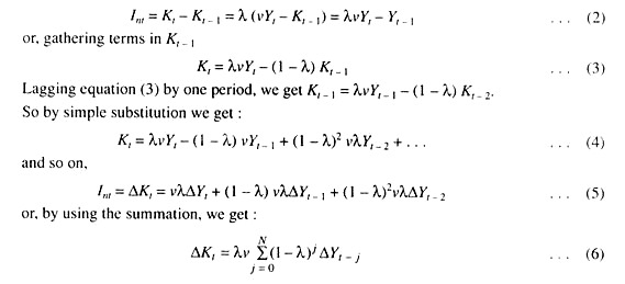
An alternative explanation of the flexible accelerator is based on expectations. Let us suppose firms base their expectations of future demand, on which their investment decisions depend, on the past levels of demand. Current investment will then be a weighted average of current and past changes in output. Let us suppose a firm is able to achieve complete adjustment, i.e., its desired stock of capital is equal to its actual capital stock. But we also assume that the desired stock of capital depends upon expected output at time t. That is

Equation (13) is similar to equation (7), the only difference being the lagged response of investment to changes in output.

Assumptions of the Accelerator Theory:

The accelerator theory of investment—in both the versions—is based on specific assumptions about the technology and factor proportions. According to this theory, the crucial determinant of investment is the level of demand or output. Relative prices, such as interest rates, wages and prices of capital goods do not play any role in determining investment.

The reason for this is that the firm, in the accelerator investment models, use fixed coefficient (Leontief-type) tech­nology which rules out the possibility of substitution of labour by capital. Fig. 4 shows that a firm is using this type of technology. The firm would then produce the desired level of output that minimised cost.

In Fig. 3 quantities of labour and capital are shown on the two axes and the fixed coefficient technology is given by the right-angled isoquants, Y₀ and Y₁. The dotted lines R₁ and R₂ passing through points denote various relative prices of capital and labour. The relative prices are irrelevant to the firm.

The minimum cost of production is at A regardless of relative factor prices. Thus, increasing the usage of capital to, say, K₂, does not yield higher output. This means that there is a unique optimum level of capital and labour needed to produce each level of output, viz., (K₀, L₁) for Y₁.

We can also suggest an alternative explanation of the consistency of capital-labour ratio. Suppose the production function is of the smooth, neoclassical type, like the one shown in Fig. 4. In this case, capital-labour substitution is theoretically possible, but can be ruled out if we make the assumption that relative prices remain constant.

If isoquants are homogene­ous of degree zero, such that a ray through the origin cuts each point of tangency between the cost constraint and the curved isoquants, the marginal rate of substitution between capital and labour remains constant at all levels of output, as is indicated by ray OY through the origin.

Overproduction:

According to accelerator principle, demand for producer goods depends on demand for consumer goods. Thus, in this case of constant or insufficiently increasing con­sumption, any augmentation of capital will lead to overproduction of consumer goods.

Inventory Investment:

The accelerator model is sometimes applied to all types of invest­ment. But it works best for inventory investment. The accelerator model of inventories assumes that inventories are proportional to a firm’s level of output. There are two reasons for this. First, when output is high, manufacturing firms need more materials and supplies on hand, and they have more goods in the process of being completed. Second, when the economy is booming, retail firms want to have more stocks of goods at their disposal to show customers. Thus, if N is the economy’s stock of inventories and Y is the output, then

N = βY

where β is a parameter showing how much inventory firms wish to hold as a proportion of output.

Inventory investment I is the change in the stock of inventories ∆N. Therefore

I = ∆N = β ∆ Y.

The accelerator model simply suggests that inventory investment is proportional to the change in output. When output rises, firms want to hold a larger stock of inventory. As a result, inventory investment is high. When output falls, firms want to hold a smaller stock of inventory. So they run down their inventory, which means that inventory investment is negative.

Since the variable Y is the rate at which the firms are producing goods, ∆Y is the ‘acceleration’ of production. And inventory investment depends on whether the economy is in the upswing (the expansion phase of the business cycle), or in the downswing (the contractionary phase).

Limitations:

The accelerator principle has obvious limitations. As Albert Aftalion stressed, production takes time, and one cannot expect capital to adjust to consumption instantaneously. Furthermore, capacity limitations impose an upper limit on the rate of gross investment at any one time, and this rate cannot be negative.