A demand curve shows how much quantity of a good will be purchased or demanded at various prices, assuming that tastes and preferences of a consumer, his income, prices of all related goods remain constant.
This demand curve showing explicit relationship between price and quantity demanded can be derived from price consumption curve of indifference curve analysis.
In Marshallian utility analysis, demand curve was derived on the assumptions that utility was cardinally measurable and marginal utility of money remained constant with the change in price of the good. In the indifference curve analysis, demand curve is derived without making these dubious assumptions.
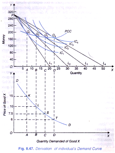
Let us suppose that a consumer has got income of Rs. 300 to spend on goods. In Fig. 8.47 money is measured on the Y-axis, while the quantity of the good X whose demand curve is to be derived is measured on the X-axis. An indifference map of a consumer is drawn along with the various budget lines showing different prices of the good X. Budget line PL1 shows that price of the good X is Rs. 15 per unit.
ADVERTISEMENTS:
As price of good X falls from Rs. 15 to Rs. 10, the budget line shifts to PL2. Budget line PL2 shows that price of good X is Rs. 10. With a further fall in price to Rs. 7.5 the budget line takes the position PL3. Thus PL3 shows that price of good X is Rs. 7.5. When price of good X falls to Rs. 6, PL4 is the relevant budget line.
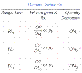
The various budget lines obtained are shown in the column 2 of the Table 8.3. Tangency points between the various budget lines and indifference curves, which when joined together by a line constitute the price consumption curve shows the amounts of good X purchased or demanded at various prices.
With the budget line PL1 the consumer is in equilibrium at point Q1 on the price consumption curve PCC at which the budget line PL1 is tangent to indifference curve IC1. In his equilibrium position at Q1 the consumer is buying OA units of the good X. In other words, it means that the consumer demands OA units of good X at price Rs. 15.
When price falls to Rs. 10 and thereby the budget line shifts to PL2, the consumer comes to be in equilibrium at point Q2 the price-consumption curve PCC where the budget line PL2 is tangent to indifference curve IC2. At Q2, the consumer is buying OB units of good X.
ADVERTISEMENTS:
In other words, the consumer demands OB units of the good X at price Rs. 10. Likewise, with budget lines PL3 and PL4, the consumer is in equilibrium at points Q3 and Q4 of price consumption curve and is demanding OC units and OD units of good X at price Rs. 7.5 and Rs. 6 respectively. It is thus clear that from the price consumption curve we can get information which is required to draw the demand curve showing directly the amounts demanded of the good X against various prices.
With the above information we draw up the demand schedule in Table 8.3 given above:
The above demand schedule which has been derived from the indifference curve diagram can be easily converted into a demand curve with price shown on the V-axis and quantity demanded on the X-axis. It is easier to understand the derivation of demand curve if it is drawn rightly below the indifference curve diagram.
ADVERTISEMENTS:
This has been done so in Fig 8.47. In the diagram at the bottom, where on the X-axis the quantity demanded is shown as in indifference curves diagram in the top pannel, but on the Y- axis in the diagram in the bottom panel price per unit of the good X is shown instead of total money. In order to obtain the demand curve, various points K, L, S and T representing the demand schedule of the above table are plotted. By joining the points K, L, Sand T we get the required demand curve DD.
In most cases the demand curve of individuals will slope downward to the right, because as the price of a good falls both the substitution effect and income effect pull together in increasing the quantity demanded of the good. Even when the income effect is negative, the demanded curve will slope downward to the right if the substitution effect is strong enough to overwhelm the negative income effect. Only when the negative income effect is powerful enough to outweigh the substitution effect can the demand curve slope upward to the right instead of sloping downward to the left.
Deriving Demand Curve for a Giffen Good:
The demand curve DD in Fig. 8.47 is sloping downward. The demand curve slopes downward because of two forces, namely, income effect and substitution effect. Both the income effect and substitution effect usually work towards increasing the quantity demanded of the good when its price falls and this makes the demand curve slope downward. But in case of Giffen good,the demand curve slopes upward from left to right.
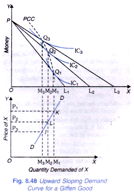
This is because in case of a Giffen good income effect, which is negative and works in opposite direction to the substitution effect, outweighs the substitution effect. This results in the fall in quantity demanded of the Giffen good when its price falls and therefore the demand curve of a Giffen good slopes upward from left to right. In Fig. 8.48 the derivation of demand curve of a Giffen good from indifferencecurves diagram is explained.
In Fig. 8.48 the Indifference curves of a Giffen good are drawn along with the various budget lines showing various prices of the good. Price consumption curve of a Giffen good slopes backward. In order to simplify the discussion in this figure we have avoided the numerical values of prices and have instead used symbols such as, P1, P2, P3 and P4 for various levels of the price of good X.
It is evident from Fig. 8.48 (the upper portion) that with budget line PL1 (or price P1) the consumer is in equilibrium at Q1 on the price consumption curve PCC and is purchasing OM) amount of the good. With the fall in price from P1 to P2 and shifting of budget line from PL1 to PL2, the consumer goes to the equilibrium position Q3 at which he buys OM2 amount of the good. OM2 is less than OM1.
ADVERTISEMENTS:
Thus with the fall in price from P1 to P2 the quantity demanded of the good falls. Likewise, the consumer is in equilibrium at Q3 with price line PL3 and is purchasing OM3 at price P3. With this information we can draw the demand curve, as is done in the lower portion of Fig. 8.48 It will be seen from Fig. 8.48 (lower part) that the demand curve of a Giffen good slopes upward to the right indicating that the quantity demanded varies directly with the changes in price. With the rise in price, quantity demanded increases and with the fall in price quantity demanded decreases.
To sum up, in most cases (that is, in case of normal goods) the demand curve of individuals will slope downward to the right, because as the price of a good falls both the substitution effect and income effect pull together in increasing the quantity demanded of the good.
Even in case of inferior goods for which the income effect is negative, the demand curve will slope downward to the right if the substitution effect is strong enough to overwhelm the negative income effect. Only in case of Giffen goods for which the negative income effect is powerful enough to outweigh the substitution effect, the demand curve slopes upward to the right intend of sloping downward to the left.


