Indifference curve analysis can be used to explain an individual’s choice between income and leisure and to show why higher overtime wage rate must be paid if more hours of work is to be obtained from the workers.
It is important to note that income is earned by devoting some of the leisure time to do some work. That is income is earned by sacrificing some leisure.
The greater the amount of this sacrifice of leisure, that is, the greater the amount of work done, the greater income an individual earns.
Further, income is used to purchase goods, other than leisure for consumption. Leisure time can be used for resting, sleeping, playing, listening to music on radios and television etc. all of which provide satisfaction to the individual. Therefore, in economics leisure is regarded as a normal commodity the enjoyment of which yields satisfaction to the individual.
ADVERTISEMENTS:
While leisure yields satisfaction to the individual directly, income represents general purchasing power capable of being used to buy goods and services for satisfaction of various wants. Thus income provides satisfaction indirectly. Therefore, we can draw indifference curves between income and leisure, both of which give satisfaction to the individual.
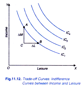
Indifference maps between income and leisure is depicted in Figure 11.12 and have all the usual properties o/indifference curves. They slope downward to the right, are convex to the origin and do not intersect. Each indifference curve represents various alternative combinations of income and leisure which provide equal level of satisfaction to the individual and the farther away an indifference curve is from the origin, the higher the level of satisfaction it represents for the individual.
The slope of the indifference curve measuring marginal rate of substitution between leisure and income (MRSLM) shows the tradeoff between income and leisure. This trade-off means how much income the individual is willing to accept for one hour sacrifice of leisure time.
In geometric terms, it will be seen from Figure 11.12 that on indifference curve IC1 at point A the individual is willing to accept ∆M(=AC) income for sacrificing an hour (∆L) or BC of leisure. Thus the trade-off between income and leisure at this point is ∆M/∆L. At different income-leisure levels, the trade-off between leisure and income varies.
Indifference curves between income and leisure are therefore also called trade-off curves.
Income-Leisure Constraint:
However, the actual choice of income and leisure by an individual would also depend upon what is the market rate of exchange between the two, that is, the wage rate per hour of work. It is worth noting that wage rate is the opportunity cost of leisure.
ADVERTISEMENTS:
In other words, to increase leisure by one hour, an individual has to forego the opportunity of earning income (equal to wage per hour) which he can earn by doing work for an hour. This leads us to income-leisure constraint which together with the indifference map between income and leisure would determine the actual choice by the individual.
The maximum amount of time available per day for the individual is 24 hours. Thus, the maximum amount of leisure time that an individual can enjoy per day equals 24 hours. In order to earn income for satisfying his wants for goods and services, he will devote some of his time to do work.
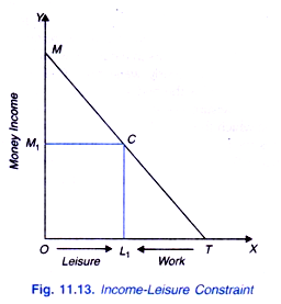
Consider Figure 11.13 where leisure is measured in the rightward direction along the horizontal axis and the maximum leisure time is OT (equal to 24 hours). If the individual can work for all the 24 hours in a day, he would earn income equal to OM. Income OM equals OT multiplied by the hourly wage rate (OM = OT.w) where w represents the wage rate.
The straight line MT is the budget constraint, which in the present context is generally referred to as income-leisure constraint which shows the various combinations of income and leisure among which the individual will have to make a choice. Thus, if a person chooses combination C, this means that he has OL1 amount of leisure time and OM1 amount of income. He has earned OM1 amount of income by working TL1 hours of work. Choice of other points on income-leisure line MT will show different amounts of leisure, income and work.
Income OM = OT. W
OM/OT = w
Thus, the slope of the income-leisure curve OM/OT equals the wage rate.
Income-Leisure Equilibrium:
ADVERTISEMENTS:
Now, we can bring together the indifference map showing ranking of preferences of the individual between income and leisure and the income-leisure line to show the actual choice of leisure and income by the individual in his equilibrium position. We will further show how much work effort (i.e. supply of labour in terms of hours worked) he would put in this optimal situation. Our analysis is based on two assumptions. First, he is free to work as many hours per day as he likes. Second, wage rate is the same irrespective of the number of hours he chooses to work.
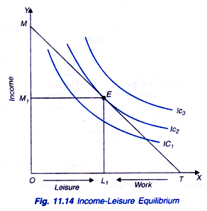
Figure 11.14 displays income-leisure equilibrium of the individual. With the given wage rate, the individual will choose a combination of income and leisure lying on the income-leisure line MT that maximises his satisfaction. It will be seen from Figure 11.14 that the given income- leisure line MT is tangent to the indifference curve IC2 at point E showing choice of OL1 of leisure and OM1 of income.
In this optimal condition, income- leisure trade off (i.e. MRS between income and leisure) equals the wage rate (i.e., that is, the market exchange rate between the two. In this equilibrium position the individual works for TL1 hours per day (TL1 = OT- OL1). Thus, he has worked for TL1, hours to earn OM1 amount of income.
Need for Higher Overtime Wage Rate:
ADVERTISEMENTS:
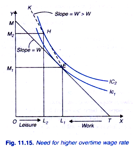
It will be interesting to know why there is need for paying higher wage rate than the normal wage rate for getting more or overtime work from the individuals. As explained above, with the given wage rate and given trade-off between income and leisure the individual chooses to work for TL1 hours per day. To do overtime work, he will have to sacrifice more leisure-time and therefore to provide him incentive to forego more leisure and thus to work for more hours it is required to pay him higher wage rate.
This is depicted in Figure 11.15 where at the equilibrium point E a steeper leisure- income line EK than MT has been drawn. TL1 is the hours worked at the wage rate w represented by the slope of the income-leisure line MT. If the higher overtime wage rate w’ represented by the line EK is fixed, the individual is in equilibrium at point H on indifference curve IC2 where he chooses to have OL2 leisure time and OM2 amount of income. Thus, he has sacrificed L1L2 more leisure to do overtime work and earns M1M2 more income than before. He now works for TL2 hours per day, TL1, at hourly wage rate wand L1L2 at higher wage rate w’. Further, he is better off than before as he is now at higher indifference curve IC2.
Wage offer Curve and the Supply of Labour:
ADVERTISEMENTS:
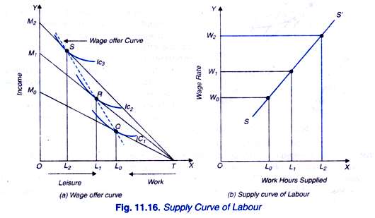
Now with the analysis of leisure-income choice, it is easy to derive supply curve of labour. Supply curve of labour shows how an individual’s work effect responds to changes in the wage rate. The derivation of supply curve of labour is depicted in Figure 11.16. In panel (a) of this figure it will be seen that at the wage rate w0 (w0 = OM0/OT), the wage line or income-leisure line is TM0 and the individual is in equilibrium at point Q where he chooses OL0 leisure time and works for TL0 hours.
That is, at wage rate w0 he supplies TL0 amount of labour. This supply of labour is directly shown against wage rate w0 in panel (b) of Figure 11.16. Now, when the wage rate rises to w1, wage line or income-leisure line shifts to TM1 (w1 = OM1/OT), the individual reduces his leisure to OL1 and supplies TL1 hours of work; L1L0 more than before (see Panel (a) in Figure 11.16). Thus, L1 number of work-hours supplied is shown against w1 in panel (b) of Figure 11.16.
Likewise, when the wage rate rises to W2 (W2, = OM2/OT), income-leisure line shifts to TM2 the individual chooses to have leisure time OL2 and supplies TL2 work-hours. In panel (a) on joining points Q, R and S we get what is often called wage-offer curve which is similar to price-consumption curve. In panel (b), the information supplied by the wage-offer curve, that is, the supply of labour (work-hours) by the individual at different wage rates is shown directly as, in this panel, supply of labour (hours worked) is measured along the X-axis and wage rate along the y-axis. A glance at panel (b) of Figure 11.16 will reveal that supply curve of labour is upward sloping indicating positive response of the individual to the rise in wage rate.
Income Effect and Substitution Effect of the Change in Wage Rate:
Now the supply curve of labour does not always slope upward as shown in Fig. 11.16. It can slope or bend backward too which implies that at a higher wage rate, the individual will supply less labour (i.e. will work less hours). Under what conditions supply curve of labour (i.e. work- hours) slopes upward and under what circumstances it bends backward can be explained in termsof income effect and substitution effect of a change in wage rate.
ADVERTISEMENTS:
As in case of change in price, rise in wage rate has both the substitution effect and income effect. The net combined effect on the supply of labour (hours worked) depends on the magnitude of the substitution effect and income effect of the rise in wage rate. It is important to note that leisure is a normal commodity which means that increase in income leads to the increase in leisure enjoyed (i.e. less work-hours supplied). That is, income effect of the rise in wage rate on leisure is positive, that is, leads to the increase in the hours of leisure enjoyed (that is, tends to decrease labour supply).
On the other hand, the rise in wage rate increases the opportunity cost or price of leisure, that is, it makes enjoyment of leisure relatively more expensive. Therefore, as a result of rise in wage rate individual substitutes work (and therefore income) for leisure which leads to the increase in supply of labour. This is a substitution effect of the rise in wage rate which tends to reduce leisure and increase labour supply (i.e. number of hours worked). It is thus clear that for an individual supplier of labour, income effect and substitution effect work in opposite directions.
Whereas income effect of the rise in wage rate tends to reduce supply of labour substitution effect tends to increase it. If the income effect is stronger than the substitution effect, the net combined effect of rise in wage rate will be to reduce labour supply. On the other hand, if substitution effect is relatively larger than the income effect, the rise on wage rate will increase labour supply.
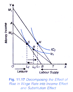
How the effect of rise in wage rate is split up into income effect and substitution effect is shown in Fig 11.17. In this figure we measure money income on the Y- axis and leisure (reading from left to right) and labour supply (reading from right to left) on the X-axis. Suppose to begin with the wage rate is W0 and if all the available hours OT are used to do work, OM0 money income is earned. This gives us TM0 as the budget constraint or which in the present context is also called leisure-income constraint. It will be seen from Figure 11.17 that TM0 is tangent to indifference curve IC1 between leisure and income at point R.
Thus, with wage rate W0 the individual is in equilibrium when he enjoys OL0 leisure and therefore he is supplying TL0 work hours of labour. Now suppose that wage rate rises to w0 with the result that income- leisure constraint line rotates to TM1. Now, with TM1 as new income-leisure constraint line, the individual is in equilibrium at point H at which he supplies TL1 work-hours of labour which are less than TL0.
Thus, with the rise in wage rate, supply of labour has decreased by L0L1. To break up this wage effect on labour supply, we reduce his money income by compensating variation in income. To do so we take away so much income from the individual that he comes back to the original indifference curve IC1. AB is such line obtained after reducing his money income by compensating variation. AB is tangent to indifference curve IC1 at point S at which he supplies TL2 hours for work.
ADVERTISEMENTS:
This shows with change in wage rate from w0 to w1, resulting in leisure becoming relatively more expensive, he substitutes work (i.e. labour supply) L0L2 for leisure. This is substitution effect which tends to increase labour supply by L0L2, Now, if the money taken from him is given back to him so that the income-leisure line again shifts back to TM1. With TM1, he reaches his old equilibrium position at point H where he supplies TL1 work- hours. Thus, movement from point S to H represents the income effect of the rise in wage rate and as a result labour supply decrease by L2L1.
Thus, while income effect of the increase in wage rate causes decrease in labour supply by L2L1 the substitution effect causes increase in labour supply by L2L1. It will be seen from Fig. 11.17 that in this case income effect is stronger than substitution effect so that the net result is reduction in labour supply by L0L1 work-hours and therefore in this case labour supply curve bends backward. Now, if substitution effect had been larger than income effect, work-hours supplied would have increased as a result of rise in wage rate and labour supply curve would slope upward.
Backward Bending Supply Curve of Labour:
It may, however, be noted that on theoretical grounds it cannot be predicted which effect will be stronger. It has, however, been empirically observed that when the wage rate is small so that the demand for more income or goods and services is very strong, substitution effect is larger than the income effect so that the net effect of rise in wage rate will be to reduce leisure and increase the supply of labour.
But when he is already supplying a large amount of labour and is earning sufficient income, further increases in wage rate may induce the individual to demand more leisure so that income effect may outweigh the substitution effect at higher wage rates.
ADVERTISEMENTS:
This implies that at higher wage rates, labour supply may be reduced in response to further rise in wage rates. This means up to a point substitution effect is stronger than income effect so that labour supply curve slopes upward, but beyond that at higher wage rates, supply curve of labour bends backward.
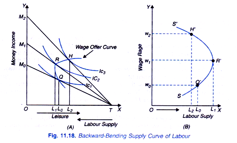
This is illustrated in Fig 11.18 where in panel (a) wage offer curve is shown, and in panel (b) supply curve of is drawn corresponding to leisure-work equilibrium in panel (a). Thus, to start with at wage rate w0 (i.e. TM0 as budget constraint) L0 amount of work-hours (labour) are supplied. This is directly plotted against the wage rate w0 in panel (b) of Fig. 11.18. When the wage rate rise to budget constraint becomes TM1 in panel (a) of Fig. 11.18 the greater amount of labour L1 is supplied.
Amount of labour L1 is directly plotted against higher wage rate w1 in panel (b) of Fig. 11.18. With the further increase in wage rate to w2, the income-leisure constraint rotates to TM2 and the individual is in equilibrium when he supplies L1 work-hours which are smaller than L1. Thus, with the rise in wage rate above w1, labour supply decreases. In other words, up to wage rate w1, labour supply curve slopes upward and beyond that it starts bending backward. This is quite evident from panel (b) of Fig. 11.18.
