
Here is a compilation of essays on ‘Production Function’ for class 9, 10, 11 and 12. Find paragraphs, long and short essays on ‘Production Function’ especially written for school and college students.
Essay on Production Function
Essay Contents:
- Essay on Production Function
- Essay on the Role of Time in Production
- Essay on Production Functions and Technology
- Essay on the Short-Run Production Function
- Essay on the Features of Production Process
- Essay on the Law of Diminishing Returns
- Essay on the Long-Run Production Function
- Essay on Production Isoquants
- Essay on the Economic Region of Production
- Essay on Optimisation in Production
- Essay on Changing Output and the Expansion Path
- Essay on Returns to Scale
- Essay on the Degree of Homogeneity of Production Function
- Essay on the Cobb-Douglas Production Function
- Essay on the Coexistence of Constant Returns to Scale and Diminishing Returns to a Factor
- Essay on Elasticity of Factor Substitution as a Property of Production Function
- Essay on Constant Elasticity of Substitution (CES) Production Function
- Essay on Linear Production Function
Essay # 1. Production Function:
ADVERTISEMENTS:
The theory of production shows how firms transform inputs into desirable outputs. In the theory of production we study how inputs or factors of production are converted into output or sale to consumers, other business firms, various government departments, and to the rest of the world. Inputs are the beginning of the production process and output is the end of the process.
The production of a commodity requires the use of two broad class of inputs-fixed and variable. A fixed input is one whose quantity cannot be readily changed when market conditions indicate that an immediate change in output is desirable. Examples of such inputs are building, machines, and managerial personnel. The supply of inputs cannot be quickly increased or decreased.
A variable input, on the other hand, is one whose quantity may be changed any time m response to desired changes in output. Examples of such inputs are various types of labour services and raw materials as also processed materials. The conversion of inputs into output depends on technology or the art (or the method) of production.
The key concept in the theory of production is the production function. The economist describes the production process in terms of a production function through which the quantities of outputs produced are functionally dependent upon the quantities of inputs used.
ADVERTISEMENTS:
The economist’s production function incorporates the engineering technology; however, its inputs and outputs usually are quantities that are bought and sold in the market place. It also incorporates a degree of optimisation. Given values for all the inputs, the production function specifies the maximum attainable value of output.
Most production functions are defined for a single output. The number of inputs depends upon the purpose for which the production function is used. Aggregate production function relates a nation’s total output to its aggregate labour and capital inputs. At the firm level a specific output such as motor cars may be related to an array of inputs such as steel, glass, types and tubes, leather, and electrical equipment, as well as direct labour and capital inputs.
A production function is a schedule (or table, or mathematical equation) showing the maximum amount of output that can be produced from any specific set of inputs given the existing technology. In short, the production function shows what outputs are associated with which sets of inputs.
A production function shows the amount of output those results from a certain amount of inputs. All production functions specify a type and amount of output, the numbers and types of inputs, and how the inputs are combined.
ADVERTISEMENTS:
Usually, there are several production functions to choose from when producing a particular good or service. A business firm often can choose among several methods to produce an output. The main factor underlying the choice is the cost of production which ultimately determines the profit of the firm.
Every production function has a cost associated with it and business firms will try to maximise the profit by using the production method that produces whatever type and quantity of product the firm wants at the lowest cost. When a firm produces a good or service using the least-cost method, efficient production and the efficient use of resources occur.
Essay #
2. The Role of Time in Production:
Time plays an important role in the theory of production. In production theory we draw a distinction between the short run and the long run. In the short run, some inputs remain fixed and the others are variable. In the long run, all inputs are variable. Thus, in the short run, changes in output occur due to changes in the use of variable factors. But, in the long run output changes when there are changes in all factors of production, including capital. In fact, all fixed factors are converted into variable factors in the long run. This is why all costs are variable in the long run.
On the basis of our knowledge of production, we develop the essential concepts of business cost. Firms have to decide what inputs to employ in production on the basis of the costs, and productivities of various inputs. Finally, we combine the theory of production and costs to show how firms decide how much output to produce. This is the basis of the theory of supply.
This means that if the producer wishes to expand output in the short run, this usually means using more hours of labour service with the existing plant and equipment. Similarly, if the producer wishes to reduce output in the short run, certain types of workers can be laid off. But it is not possible to sell a machine or discharge a building, even when its use may fall to zero.
In the long run, a firm-produces more output in a more efficient way (i.e., at a lower cost than in the short run. For example, in the short run, a producer may be able to expand output only by operating the existing machine or plant more intensively (i.e., by using it for longer hours per day). This, of course, entails paying higher overtime wages to workers. In the long run, it may be more economical to create additional production facilities and return to the normal workday.
Essay #
3. Production Functions and Technology:
ADVERTISEMENTS:
The conversion of inputs into output depends on technology. Technology is the knowledge that we possess about production processes. However, technology does not remain constant over time. Technology improves as companies invest on scientific research. Technological change in the form of production and process innovation has a significant influence on production functions.
Technology determines how we do things and it affects the design of process and machinery and equipment and influences inventory control, packing, human relations, purchasing and virtually every aspect of production. Technological changes are leading to more efficient ways to produce and distribute almost everything.
Technology defines the range of production methods from which a business can choose: from old methods to the latest ones. As technology grows and new ideas are developed, some processes and equipment become obsolete. This is known as creative destruction, a term coined by J. A. Schumpeter.
New machinery, production processes and other results of technological change frequently replace the old, causing some industries to grow and prosper and others to shrink and perhaps ultimately disappear. For example, the introduction of robotics into assembly lines has not only affected the demand for labour, but has also caused much of the machinery and equipment in automobile plants to become obsolete.
ADVERTISEMENTS:
Thus, technological progress is both an opportunity and a threat. Creative destruction also occurs at the international level when firms in one country lags behind competing firms in other countries which use modern improved technology.
Essay #
4. The Short-Run Production Function:
The short-run production function gives us the total (maximum) output which can be obtained from different amounts of the variable input (such as labour), given a specified amount of the fixed input (and, of course, the required amounts of raw materials or ingredient inputs).
The short run production function is written as:
ADVERTISEMENTS:
Q = f (K, L) = f (L)
since K is held constant.
This means that output (Q) or total product is a function of labour (L) alone, capital remaining fixed. The short-run production function shows how total product responds to an increasing application of the variable factor (labour). Table 1 illustrates a short-run production function.

In the first column we show labour input and in the second column we show total output. In the third and fourth columns we show APL and MPL respectively.
Average Product:
ADVERTISEMENTS:
The average product of an input (such as labour) is total product divided by the amount of the input used to produce this output. Thus, average product is the output- input ratio for each level of output and in this case it is expressed as APL = Q/L.


Marginal Product:
The marginal product of an input (such as labour) is the addition to the total product attributable to the addition of one unit of the variable input to the production process, the fixed input (capital) remaining unchanged. In this case, it is expressed as
MPL = dQ/dL
ADVERTISEMENTS:
In Fig. 1 we show the total product curve and in Fig. 2 we show the average and marginal product curves. These curves are drawn on the basis of production data presented in Table 1.
Essay #
5. Features of the Production Process:
Table 1 and Fig. 1 and Fig. 2 illustrate some important features of the short-run production process:
(i) Total Product:
Total product initially increases at an increasing rate, then at a decreasing rate, then becomes maximum and, ultimately, falls. For this reason, both APL and MPL initially rise, reach a maximum, and then decline. In an extreme situation, APL could fall to zero because total product itself may fall to zero. MPL, on the other hand, may actually become negative.
In fact, MPL of agricultural workers in some less developed countries—such as India, Pakistan and Bangladesh, is, in fact, negative. Workers are so many in number that an additional worker may just cause the total product to fall by standing in others’ way (i.e., creating a disproportionate crisis) in which case MPL is negative.
ADVERTISEMENTS:
In Table 1, the MPL is negative because it (the variable input) is used too intensively with capital (the fixed input). Suppose a machine can be operated for 24 hours. Each worker is supposed to operate it for 8 hours a day.
If 3 workers are employed, the factor proportion will be optimal. But if 6 workers are employed, each will be able to use the machine for only 4 hours a day so during the remaining 4 hours, he has to remain idle and his productivity is bound to fall. He may even cause total product to remain constant or even fall, in which case the MPL is negative.
(ii) The relation between MPL and APL:
A second notable feature of the short-run production process is that MPL exceeds APL when APL is rising, equals APL when APL is maximum (constant) and is less than APL when APL is falling. The relation between ‘margin’ and ‘average’ is mathematical. Consider a cricket player who has an average score of 85 in four test matches. If his score of the fifth test exceeds 85, then the average rises. If it is below 85, the average falls. The same marginal-average relationship is found in production.
So long as MPL > APL, APL must increase. If MPL < APL, APL must fall. The two curves must intersect at point N where APL is maximum, because an MPL equal to APL does not change the APL.
Thus, we see that both APL and MPL rise first, reach a maximum and decline thereafter. When APL attains its maximum, APL = MPL. The relations hold only in case of a variable- proportions production function.
ADVERTISEMENTS:
From Table 1, we can discover three stages of the production process in the short run. In the first stage MPL falls; in the second stage APL falls; and, in the third stage, total product also falls.
Essay #
6. The Law of Diminishing Returns:
The shape of the MPL curve in Fig. 2 illustrates an important principle: the ‘law of diminishing marginal returns’. From Table 1 we see that when the second worker is employed, MPL increases from 10 to 12. This happens because the capital-labour ratio is high.
Eventually, however, as the input ratio declines, the MPL must also decline. When the number of workers increases, each worker has, on the average, fewer units of the fixed input (capital) to work with. Initially, when the fixed input is relatively abundant, more intensive utilisation of the fixed input by the variable input may increase the MPL.
However, a point is ultimately reached beyond which an increase in the intensity of use of the fixed input yields progressively less and less additional returns. From Table 1 we see that, as more and more workers are employed, MPL first diminishes, then falls to zero, and, ultimately, becomes negative.
Thus, using the short-run production function we can understand one of the most famous laws of economics—the law of diminishing returns. The law states that we will get less and less extra output when we add additional doses of an input while holding other inputs fixed. Alternatively stated, the marginal product of each unit of input will decline as the amount of that input increases, holding all other inputs constant.

There are two interpretations of the law of diminishing returns. Successive equal increments of the variable factor applied to the fixed factor(s) yield progressively less and less increments in total output.
Increasingly larger increments of the variable factor must be applied to the fixed factors in order to yield constant increments in total output.
The law of diminishing returns expresses a simple truth or fact of economic life. As more of an input such as labour power is added to a fixed amount of land, machinery, and other inputs, each unit of labour (i.e., each worker) gets less and less of the complementary factor to work with. There is pressure on land due to overcrowding. The machinery is overworked and the marginal product of labour declines.
Essay #
7. The Long-Run Production Function:
Thus far we have taken labour as the only variable factor. Therefore output was treated as function of labour input alone, capital and other inputs remaining fixed. Now, in the long run, when factors are variable, production function can be expressed as
Q = f (K, L, etc.).
For the sake of simplicity we assume that output (Q) is a function of capital (K) and labour (L), i.e., we consider a production function which involves the use of only two inputs. However, the same analysis can be extended to cover any number of inputs. So the production function is written as Q = f (K, L).
Now, since K and L are freely substitutable there are different combinations of K and L which can be used to produce the same output. It is the task of the entrepreneur or the production manager to select the particular input combination which minimizes the cost of producing any given level of output. We may now discuss how this is done.
Two related points are to be noted in this context. The long-run production function explains how to achieve the maximum productivity at a given cost. Alternatively, it allows us to understand how firms choose input allocations from a wide range of possibilities.
Essay #
8. Production Isoquants:
The long-run production possibility of a firm is illustrated by drawing isoquants. These are a producer’s indifference curves. While a consumer’s indifference curves show the different levels of utility (which cannot be measured), a producer’s isoquants show different levels of output(which can be measured).
Table 2 shows a firm’s long-run production possibilities. We see that there are three different ways of producing a fixed level of output (100 units), as shown by the three possibilities (A, B, C). We can also consider various other possibilities.
If we plot this information graphically, we get a firm’s isoquant which represents its long-run production function involving the use of only two variable factors. By using this technique we can show three variables, viz., output, capital and labour in a two-dimensional diagram.

In Fig. 4, Q = 100 is a typical isoquant. It is the locus of points such as A, B, C, showing alternative combinations of K and L which can yield the same level of output (100). Thus, an isoquant represents different inputs combinations or input ratios that may be used to produce a certain specified level of output.
Alternatively stated, an isoquant is a curve in input space showing all possible combinations of inputs typically capable of producing a given level of output. Iso means ‘constant’ and quant means ‘quantity’. This is why an isoquant is also called an equal product curve. For movements along an isoquant the level of output remains constant and the input ratio (called factor proportion) changes continuously. For example, at point A, the production process is capital intensive and at point C, it is labour intensive.
Along a ray through the origin such as OA, OB, or OC, various levels of output can be produced by using the same input ratio. In Fig. 4 we have drawn three isoquants showing three different output levels. All the isoquants together constitute the isoquant map of the producer. It is quite obvious that an isoquant such as Q2, which is above another isoquant such as Q, shows a higher level of output. Similarly, the isoquant Q3 shows a still higher level of output than Q2.

Fixed-Proportion Production Function:
Using isoquants, we can illustrate the case of fixed-proportion production function. Production is subject to fixed proportions when one— and only one—combination of inputs can produce a specified output. Such a production function is represented as
Q = min. [(K/ (α), (L/ (β)]
where α and β are constants and ‘min.’ means that Q equals the smaller of the two ratios. Such a production function is shown in Fig. 5. In this case, there is only one ray through the origin OR. The isoquants are also L-shaped.
This means that if three units of labour and two units of capital are employed; 100 units of output can be produced; so, to produce 200 units of output, the inputs are also to be doubled. Thus, this production function exhibits constant returns to scale (a term to be defined later in this essay). Returns to scale are studied statistically.

A more realistic case is that in which many-but not an infinite number of distinct fixed-proportions processes are available. For example, in Fig. 6 four different fixed-proportion processes are available to produce 100 units of a commodity. The kinked line ABCDE is different from a ‘normal’ smooth isoquant shown in Fig. 6. The reason is that no input combination lying on the arc between A and B, B and C, etc. is itself a direct feasible input combination.

Input Substitution:
Perhaps the most notable characteristic of production under conditions of variable proportions —or a large number of alternative fixed-proportion processes—is that some specified level of output can be produced by using different combinations of inputs. This means that one input can be substituted by the other, keeping output constant.
Marginal Rate of Technical Substitution:
The long-run production process permits input substitution. In fact, the isoquant shown in Fig. 7 slopes downward from left to right due to the law of substitution which states that the usage of one input is always at the expense of the other. Suppose the producer is initially at point a on Q1, producing 150 units of output.
Now suppose, through mistake, he moves from point a to b, which is on a lower isoquant. As a result, output falls from 150 to 100 units. The reason is that he is using the same amount of labour but less capital, so, to keep his output constant, he has to use more capital, i.e., he has to move from b (which is on Q1) to c (which is on Q2).
This point may now be explained.
In this case:
Output lost (by moving from a to b) is = output gained (by moving from b to c)
or , – ∆K.MPk = ∆L.MPL
Suppose he reduces the use of capital by 5 units by moving from a to b and MPK is 10; so output falls by 50 units (from 150 to 100). If MPL = 5, 10 units of labour are to be used to keep output constant. Suppose 1 unit of capital is one machine and one unit of labour is one worker.
This means that 1 machine is as productive as 2 workers (i.e., 1 machine can do the same job which can be done by two workers).
Then the slope of the isoquant is
![]()
This is known as the marginal rate of technical substitution (MRTS) of labour for capital, or the desired rate of factor (input) substitution. It is the rate at which a producer wants to substitute one factor by another, holding his output constant.


Alternatively stated, the MRTS measures, the reduction in one input (K) per unit increase in the other (L), i.e., just sufficient to maintain a certain fixed level of output. The MRTS at a point on an isoquant is equal to the negative of the slope of the isoquant, at that point. It is also equal to the ratio of the marginal product of labour to marginal product of capital. This important point is illustrated in Fig. 8.
Here we evaluate MRTSLK at a point of the isoquant Q1 and not over a segment of the isoquant, as we have done in the context of Fig. 4. At point C in Fig. 8, output remains fixed at 100. So we can write
Output lost +Output gained = 0
– dK. MPk + dL. MPL = 0
– ![]()

Thus, the slope of an isoquant is the ratio of two absolute changes—absolute change in L and absolute change in K. Since one of the two changes is negative, MRTS is always negative. AM MRTS is the ratio of the two marginal products, i.e., MPL and MPK. It is, in fact, the desired rate of factor substitution, i.e., the rate at which the producer wants to substitute one factor by the other, while holding the output level constant.
The Convexity of Isoquants:
Isoquants are not only downward sloping from left to right. They are also convex to the origin due to diminishing MRTS. This means that the desired rate of input substitution or the absolute value of ∆K/∆L itself decreases as the producer moves along the same isoquant and uses more labour (capital) and less capital (labour) by moving from left to the right (or from right to left) along the same isoquant.
As capital is substituted by labour, the MPL declines while MPK increases. Hence the MRTSLK declines as labour is substituted for capital so as to maintain a constant level of output. Diminishing MRTS implies that an isoquant must be convex. In Fig. 9, A, B, C, and D are four input combinations lying on the isoquant Q1. Point A has the combination K1 units of capital and L1 unit of labour; B has K2 units of capital and L2 units of labour.
For movement from A to B, the MRTS is
![]()
Likewise, for movements from B to C and C to D, the marginal rate of technical substitution are K2 – K3 and K3 – KA, respectively. Due to diminishing MRTS, K1– K2> K2– K3> K3– K4. The amount of capital replaced by successive units of labour will decline if and only if the isoquant is convex. Since the amount must decline, isoquant must be convex. This is so because the two inputs are not perfect substitutes of each other.
If they are perfect substitutes in production, then one can be substituted by the other at the same rate throughout. In this case, an isoquant will be a straight line with constant MRTS as shown in Fig. 10(a). And if MRTS increases, an isoquant will be concave to the origin as shown in Fig 10(b).


Essay # 9
. Economic Region of Production:
It is a well-known proposition that a consumer’s indifference curve cannot have upward sloping segments due to the existence of bliss point. However, isoquants may have positively sloped segments as shown in Fig. 11. This means that they may bend back upon themselves.

Economic and Uneconomic Regions of Production:
There is some similarity between the theory of consumer demand and the theory of production. However, there is one notable difference also. Since utility cannot be measured and negative utility does not carry any economic sense consumer indifference curves do not have positively sloped regions. Positively slopes regions of indifference curves are ruled out due to the existence of bliss point. But output can be measured and the slope of the isoquants indicates the behaviour of the marginal product of the two variable factors. Therefore, production isoquants may have both negatively and positively sloped regions.
Normally isoquants are downward sloping. As we move along the same isoquant from left to right we use more labour and less capital, holding output constant. But in Fig 11 we see that isoquants have both upward-sloping and backward-bending regions
The upward-sloping region in Fig. 11 occurs when we have diminishing total returns to labour and MPL = 0. The backward bending region occurs when we have diminishing total returns to capital and MPK = 0.
A firm that wants to minimise its costs of production should never operate in the region of upward sloping or backward-bending isoquants. For example, a producer should not operate at point like D where MPL = 0. The reason is that it could produce the same output but at a lower cost by producing at point C.
By producing in the range where MPL = 0, the firm would be wasting money by spending it on unproductive labour. For this reason we refer to the region in which isoquants slope upward as uneconomic region of production. In contrast, the economic region of production is the region of downward-sloping isoquants.
Ridge Lines:
To separate the two regions of production we draw ridge lines. The locus of points of isoquants where the marginal products of the factors are zero form the ridge lines. The area enclosed by two ridge lines is called the economic region of production and the area outside the ridge lines is uneconomic region of production.
There are two ridge lines because there are two variable factors. The upper ridge line implies that the MPk = 0 or negative at any point above it. The lower ridge lines imply that the MPL = 0 or negative at any point to the right of it. Production techniques are only (technically) efficient inside the ridge lines. Outside the ridge lines the marginal products of the factors are zero or negative and the methods of production are inefficient, since they require more of both factors for producing a given level of output.
Such inefficient methods are not considered by the theory of production, since they imply irrational behaviour of the firm. The condition of positive but declining marginal products of the factors defines the range of efficient production (the range of isoquants over which they are convex to the origin.)
Essay #
10. Optimisation in Production:
It may be noted that the isoquant expresses the desire of the producer, i.e., what he is willing to produce. But the desire to produce a certain level of output, such as 150 units, is not enough. The producer must have the capacity to do so. And his capacity to produce depends on his budget (when technology remains unchanged), which is shown by his isocost line. Now a rational producer whose objective is profit maximisation has two alternatives which are presented:
Alternative 1: Output Maximisation Subject to Cost Constraint:
Suppose a producer has a fixed budget of Rs. 300. With this fixed sum of money he will try to produce as much output as possible. A rational producer will always try to reach the highest attainable isoquant permitted by the isocost line. In Fig. 13, with the isocost line AB the producer can reach Q2 and produce 150 units of output by spending, say, Rs. 300. This is the maximum amount of output he is capable of producing due to resource (budget) constraint. In this case, his cost per unit is Rs. 300/150 = Rs. 2.
Can he produce more output and reduce his unit cost further? Obviously not. [With the isocost line AB he cannot reach Q3 and produce 200 units of output.] If, through mistake, he moves to point For G along the same isocost line (AB) his cost will remain the same but his output will fall to 100 units. So his cost per unit will rise to Rs. 300/100 = Rs. 3. This point may be explained further.

At point F, the slope of the isoquant Q1, as is indicated by the dotted line which is tangent to point F, is greater than the slope of the isocost line. Suppose the entrepreneur thought of producing at point F. The MRTSLK given by the slope of the tangent TT’ is relatively high. Suppose it is 2: 1, implying that one unit of labour can replace 2 units of capital at that point. The relative input price, given by the slope of AS, is much less, say 1: 1.
In this case, 1 unit of labour costs the same as 1 unit of capital but it can replace 2 units of capital in production. The producer would obviously be better-off by substituting labour for capital. The opposite argument holds good at point G, where the MRTSLK is less than the input price ratio.
So long as the two are not equal, the producer can achieve either a greater output or a lower cost by moving in the direction of equality. So only point E is economically feasible because it ensures maximum amount which implies minimum cost per unit. And the combination of K and L corresponding to point E (viz., K2 and L2) is known as the least cost combination of inputs.
At point E we see that the slope of the isoquant Q2 is the same as the slope of the isocost line, or, MRTSLK (the desired rate of factor substitution) = w/r (actual rate of factor substitution)
This is the condition of producer’s equilibrium or optimisation in production.
Alternative 2: Cost Minimisation Subject to Output Constraint:
Now suppose the producer’s objective is to produce exactly 150 units of output (neither one unit more nor one unit less). The producer will try to produce this target level of output at the lowest possible cost. For any given level of output, cost minimisation refers to the choice of input combination which yields the smallest possible total cost. This allocation is illustrated in Fig. 14. Here there is only one isoquant Q2 (showing an output level of 150 units). But there are three isocost lines.

If the producer’s budget is C1 = Rs 200, he will be on A1 B1. With this isocost line he cannot attain the desired level of output. So he has to increase his budget to at least C2= Rs 300. This will enable him to reach the isoquant Q2 and produce 150 units of output at a unit cost of Rs 2, as was the case under alternative-1. Since at this point MRTS = FRP, cost cannot be reduced further (i.e., the producer is in equilibrium in the input market).
If by mistake the producer moves to point F or point G, his output will remain the same but his total cost will be C3 = Rs 450 and his cost per unit will be Rs 450 / 150 = Rs 3. Once again he becomes a high cost producer by moving to the right or to the left of point E. So only point E is economically feasible and the combination of K and L corresponding to this point (viz., K2 and L2 is the least cost combination of inputs. So our main prediction here is:
A rational producer whose objective is output maximisation subject to cost constraint or cost minimisation subject to output constraint will choose the least cost combination of inputs. Once this input combination is chosen, cost cannot be reduced further.
The tangency condition for cost minimisation yields the result that the input combination which minimizes the total cost of producing any given level of output must necessarily satisfy the equality of the ratio of marginal product of any two factor inputs with the ratio of their prices. Thus, output maximisation subject to cost constraint or cost minimisation subject to output constraint yields identical result. This is known as the duality of production and cost.

Essay #
11. Changing Output and the Expansion Path:
In the long run, the producer may want to expand output by increasing his scale of production, i.e., by increasing the using of all the factors proportionately. So the producer’s equilibrium points will change. This point is illustrated in Fig. 15.

With fixed input prices, the output corresponding to isoquant Q1 can be produced at a minimum cost at point E, where the isoquant is tangent to the isocost line A1B1. With input prices remaining constant, suppose the producer wants to expand output to Q2. The new equilibrium is found by shifting the isocost line to A2B2 until it is tangent to Q2 at point F.
Similarly, if the producer wishes to expand output to g3, production would be at point G or Q3 on A3B3. By connecting points E, F, G, etc. we get the expansion path of the firm OR. For given input prices, the curve indicates what the firm’s will be in terms of factor input combinations. It is a locus of successive cost minimising points (i.e., at each point MRTSLK =w/r).
The expansion path is the path along which output will expand when factor prices remain constant. The expansion path then shows how factors proportions change when output or expenditure changes, input prices remaining constant throughput. In Fig. 15(a), OR is the expansion path for a general production function.
In Fig. 15(b), the straight line expansion path OR is one for a specific production function. This is the expansion path for a homogeneous production function. We shall refer to this type of production function later in this essay.
Essay #
12. Returns to Scale:
When inputs have positive marginal products, a firm’s total output must increase when the quantity of all the inputs are increased simultaneously, i.e., when a firm’s scale of operation increases. We often want to know by how much output will increase when all inputs are increased by a certain percentage.
For example, by how much would a construction company be able to increase its output if it doubled its man-hours of labour and its machine-hours of capital? The concept of returns to scale tells us the percentage increase in output when a firm increases all of its input quantities by a certain percentage amount:
![]()
To illustrate returns to scale, suppose a firm owns two inputs—labour (L) and capital (K) — to produce its quantity of output Q. Now suppose all the inputs are increased by the same proportionate amount λ > 1 (i.e., the quantity of labour increases from L to λL and the quantity of capital increases from K to λK). Let .s represent the resulting proportionate increase in the quantity of output (i.e., the quantity of output increases from Q to sQ).
Then:
1. If s > λ, we have increasing returns to scale, in which case a proportionate increase in all inputs leads to a more-than-proportionate increase in output.
2. If s = λ, we have constant returns to scale, in which case a proportionate increase in all inputs leads to an exact proportionate increase in output.
3. If s < λ ,we have decreasing returns to scale, in which case a proportionate increase in all inputs leads to a less-than-proportionate increase in output.
There are three ways of showing returns to scale, viz., from the expansion path, from output elasticity and from the degree of homogeneity of the production function.
First we show returns to scale from the expansion path.
Fig. 16(a) illustrates increasing returns to scale: if the quantity of labour and capital are doubled, output gets more than doubled.
Fig. 16(b) illustrates constant returns to scale: doubling the quantity of labour and capital doubles the quantity of output.
Fig. 16(c) illustrates decreasing returns to scale: doubling the quantity of capital and labour less than doubles output.


Importance of the Concept:
The concept of returns to scale has practical relevance. When a production process exhibits IRS, there are cost advantages from a large-scale operation. In particular, a large firm would be able to produce a given amount of output at a lower cost per unit than could two small firms of equal size, each producing exactly half as much output. The reason is that, with IRS, the large firm needs to employ less than twice as many units of labour and capital as the smaller firm to produce twice as much output.
If a large firm enjoys such a cost advantage over smaller firms, a market would be most efficiently served by one large firm than several small firms. This cost advantage of large-scale production provides a justification for allowing firms to operate as natural monopolies in markets as electric power and postal services.
Elasticity of Production (Output Elasticity):
Returns to scale can also be found out from the elasticity of production. It is defined as the ratio of the proportionate change in output to the proportionate change in factor inputs and in case of two variable factors it is expressed as:
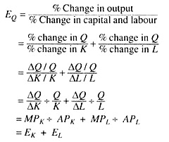
where EK is the output elasticity of capital and EL is the output elasticity of labour. The sum of the two output elasticities is called the coefficient of the production function (FC).
If EQ > 1, the production function exhibits IRS since a certain percentage increase in both K and L leads to a more than proportionate increase in Q.
If EQ = 1, the production function shows CRS since a certain percentage increase in both K and L leads to an exactly proportionate increase in Q.
If EQ < 1, the production function exhibits DRS since a certain percentage increase in both K and L leads to a less than proportionate increase in Q.
Essay #
13. The Degree of Homogeneity of Production Function:
A special type of production function is homogeneous production function. A production function is said to be homogeneous of degree n if the multiplication of all the independent variables of the function by a positive constant such as λ results in the multiplication of the dependent variable of the function by a term λn. Here n is the degree of homogeneity of the function.
The function is written as:
λnQ = f (λK, λL).
Now if n > 1, λn > λ, and the production function shows IRS.
If n = 1, λn = λ, and the production function shows CRS.
In this case the production function is called linearly homogeneous.
And if n < 1, λn < λ, and the production function shows DRS.
Homothetic Production Function:
Another production function is homothetic production function. For such a production function the ratio of MPL to MPK remains constant for a proportionate increase in L and K. An isoquant map for a linearly homogeneous production function is shown in Fig. 17. Consider any ray through the origin, say OR, which specifies a capital- labour ratio. This ray intersects all isoquants at points such as E,F so that the slopes of the isoquants are the same, i.e., the MRTSLK is the same at all those points.
This is true of any ray through the origin and not just OR. This means that a single isoquant fully describes the isoquant map when the production function is homogeneous of degree one. Thus, a production function having this property (that is, the MRTS is the same along any ray through the origin) said to be homothetic.

It may be noted that linearly homogeneous production functions are homothetic but the converse is not true: there are homothetic production functions that are not linearly homogeneous.
Essay #
14. The Cobb-Douglas Production Function:
There is a production function that is intermediate between a linear production function and a fixed proportion production function. This production function is known as the Cobb-Douglas production function and is written as
Q = ALα Kβ
where A, α, and β are possible constants. Here A is efficiency parameter, showing the effect of technology on production.
Let L1, K1 denote the initial quantities of labour and capital and let Q1 denote the resulting value of output. So,
Q1=AL1 αK1β
Now let us increase all input quantities by the same proportional amount λ.
λ > 1 and let Q2 denote the resulting value of output:
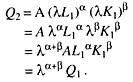
Now if α + β > 1, then λα+β > 1, and so Q2 > λQ1. Then the production curve shows IRS.
If α + β = 1, it shows CRS and if α + β < 1, the production function exhibits DRS.
Thus, the sum of the two exponents α and β determines the degree to which returns to scale are increasing, constant or decreasing.
Essay #
15. Coexistence of Constant Returns to Scale and Diminishing Returns to a Factor:
We have studied two laws of production so far, viz., the law of variable proportions (which holds in the short run) and the law of returns to scale (which holds in the long run). It may be noted that there is no logical contradiction between the two laws. The law of diminishing returns is universally applicable.
So every short-run production function shows diminishing returns. And the same production function which exhibits diminishing returns in the short run may also exhibit any of the three stages of the production process in the long run. This point is illustrated in Fig. 18.

Constant Returns to Scale vs. Diminishing Marginal Returns to a Factor:
It is important to understand the distinction between the concept of returns-to scale and diminishing marginal returns. Returns to scale pertain to the impact of an increase in all input quantities simultaneously, while diminishing marginal returns pertain to the impact of an increase in the quantity of a single input, such as labour holding the quantities of all of the other inputs fixed.
Fig. 18 illustrates this distinction. If we double the quality of labour, from 10 to 20 units per year, holding the quantity of capital fixed at 10 units per year, we move from point A to B and output goes up from 100 to 140.
If we then increase the quantity of labour from 20 to 30, we move from point B to C. Output goes up to some extent, but only to 170. In this case, we have diminishing marginal returns to labour: the increase in output brought about by a 10-unit increase in the quantity of labour goes down as we employ more and more labour.
In contrast, if we double the quantity of both labour and capital from 10 to 20 units per year, we move from A to D and output doubles from 100 to 200 units per year. If we triple the quantity of labour and capital from 10 to 30, we move from point A to E, and output triples from 100 to 300 units. For the production function in Fig. 18, we have CRS but diminishing marginal returns to labour.
If the production function is homogeneous of degree one:
(1) There is CRS, that is a proportional expansion of all inputs expands output by the same proportion and
(2) The marginal and average products depend only on the ratio in which the inputs are combined and, in particular, they are independent of the absolute amounts of the inputs employed.
Essay #
16. Elasticity of Factor Substitution as a Property of Production Function:
Finally we refer to the elasticity of substitution since it is a property of production function. It is a measure of the ease or difficulty of substituting capital for labour in response to a change in the ratio of prices of labour and capital.
The term was introduced by J. R. Hicks in 1932 (in his Theory of Wages).
Hicks’ definition goes as:
The elasticity of substitution measures the relative responsiveness of the capital-labour ratio to given proportional changes in the MRTSL,K. This definition suggests that the capital-labour ratio is a well-defined function of the MRTS. This is true when the production function is homothetic.
The formula for elasticity of substitution (σ) is:
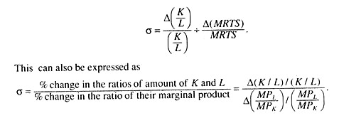
The denominator in the above expression is the MRTS. Essentially, the elasticity of substitution is the change in factor proportion (numerator) in relation to their MRTS (the denominator). The above expression may be illustrated graphically using isoquants and process rays. See Fig. 19.
The numerator of the above expression is the percentage change in factor proportion when moving from process ray OR1 to process ray OR2. The denominator is the change in each factor’s marginal product given by the slope of the isoquant at the point of tangency A and B.

In equilibrium, MRTS will be equal to w/r. Hence σ can also be expressed as the elasticity of K/L wrt w/r
![]()
Thus, the elasticity of substitution shows the proportional change in the capital-labour ratio induced by a given proportional change in the factor-price ratio. When no input substitution is possible, i.e., inputs must be used in fixed proportions σ = 0, where factors are perfect substitutes, σ → ![]() . The actual measure will lie somewhere between the two.
. The actual measure will lie somewhere between the two.
When it is one, as exhibited in the Cobb-Douglas production function, labour can be substituted for capital in any given proportion, and vice versa, without affecting output. This means that a given percentage increase in the ratio of the price of labour to the price of capital causes an equiproportional increase in the capital-labour ratio.
Essay #
17. Constant Elasticity of Substitution (CES) Production Function:
The constant elasticity of substitution (CES) production function provides a generalisation of the Cobb-Douglas production function. The CES production function is a linearly homogeneous production function with a constant elasticity of input substitution. This elasticity can take value other than unity.
The actual form of the production function is:
Q = A[αK-p + (1 – α)L-p ] -1/p
where Q is output, A is the efficiency parameter, K and L are capital and labour, α and (1 – α) are the distribution parameters and p is the substitution parameter. If σ = 1, the CES production function tends to the Cobb-Douglas production function.
Essay # 18
. Linear Production Function:
Linear—some called fixed-coefficient—production functions are frequently used. If it is assumed that a and b units of labour and capital, respectively, are required to produce 1 unit of output, then the linear production function is given by
Q = min. (L/a, K/b)
Direct substitution between the two factors is not possible. Each of the factors may be limiting. However, substitution between labour and capital is sometimes achieved by allowing the simultaneous use of several distinct linear processes for the production of a particular good.