
Let us suppose that a firm uses two inputs, labour (L) and capital (K), to produce its output (Q), and its production function is
Q = f(L,K) (8.122)
[where L and K are quantities used of inputs labour (L) and capital (K) and Q is the quantity of output produced]
The function (8.122) is homogeneous of degree n if we have
ADVERTISEMENTS:
f(tL, tK) = tn f(L, K) = tnQ (8.123)
where t is a positive real number.
In the theory of production, the concept of homogenous production functions of degree one [n = 1 in (8.123)] is widely used. These functions are also called ‘linearly’ homogeneous production functions.
If the production function (8.122) is linearly homogeneous, then we would have
ADVERTISEMENTS:
f(tL, tK) = tf(L, K) = tQ (8.124)
From (8.124), it is clear that linear homogeneity means that raising of all inputs (independent variables) by the factor t will always raise the output (the value of the function) exactly by the factor t. Assumption of linear homogeneity, therefore, would amount to the assumption of constant returns to scale in economic theory.
Let us discuss below the properties of a linearly homogeneous production function as defined by (8.122) and (8.124).
Property I:
The average (physical) product of labour (APL) and of capital (APK) can be expressed as functions of capital-labour ratio (K/L).
ADVERTISEMENTS:
To prove this, let us multiply L and K in (8.122) by the factor t = 1/L. Then owing to linear homogeneity, we would have
f(L/L, K/L) = Q/L
⇒ f [(1,K/L)] = Q/L
⇒ g (K/L) = APL (8.125)
Similarly, we would have
Q/K = h(L/K)
⇒ APK = h (L/K) (8.126)
Eqns. (8.125) and (8.126) give us that if L and K are increased by the firm in the same proportion, keeping the K/L ratio constant, then there would be absolutely no change in APL and APK, i.e., the APL and APK functions are homogeneous of degree zero in L and K.
Property II:
The marginal physical products, MPL and MPK, are also the functions of the K/L ratio.
ADVERTISEMENTS:
We may establish this in the following way.
Q = L.g (K/L) [from (8.125)] (8.127)
Therefore, we have
MPL = ∂Q/∂L = g (K/L) + L.g’(K/L)(−K/L2)
ADVERTISEMENTS:
= g(K/L) – (K/L)g’(K/L)
= Ψ (K/L)
Also, from (8.127), we have
MPK = ∂Q/∂K = Lg’(K/L) (1/L)
ADVERTISEMENTS:
= g’ (K/L)
(8.128) and (8.129) establish Property II. That is, if the production function is homogeneous of degree one, then both MPL and MPK are homogeneous functions of K and L of degree zero.
Property III:
For the homogeneous production function of degree one as given by (8.122) and (8.124) we would have
We may establish this property in the following way. From (8.128) and (8.129), we have
L(∂Q/∂L) + K (∂Q/∂K) = Q
ADVERTISEMENTS:
We may establish this property in the following way.
From (8.128) and (8.129), we have
L(∂Q/∂L) + K (∂Q/∂K)
= Lg (K/L) –L (K/L)g’(K/L) + Kg’(K/L)
= Lg (K/L) – Kg’ (K/L) + Kg’(K/L)
= Lg(K/L) = Q [from (8.127)] (8.130 )
ADVERTISEMENTS:
(8.130) establishes property III, also known as the Euler’s Theorem.
This property may also be stated like this. If the inputs labour (L) and capital (K) are paid at the rate of their respective marginal products (∂Q/∂L and ∂Q/∂K) then the total product (Q) would be exhausted, provided the production function is homogeneous of degree one.
Property IV:
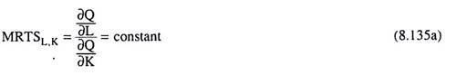
The MRTS in the case of a homogeneous production function (of any degree n) is a function of K/L ratio, and the expansion path for such a function will be a straight line.
From (8.122) and (8.123), we have
Q = f(L, K)
and f(tL, tK) = tnQ.
ADVERTISEMENTS:
where t is a positive real number.
Since (8.122) has been assumed to be a homogeneous production function of degree n, we have got (8.123).
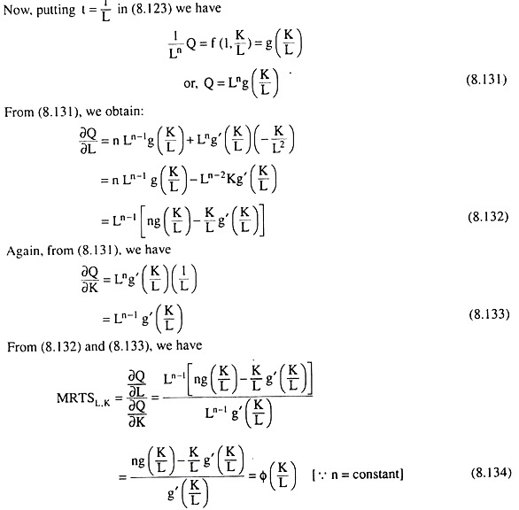
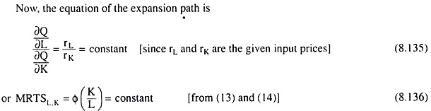
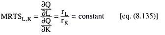
That is, along the expansion path MRTSL,K = φ (K/L) = constant, i.e., along this path ratio is constant which implies that the expansion path is a straight line from the origin. Hence, Property IV is established. It may be noted that if we put n = 1 in above calculations, we would be able to establish the property when the production function is linearly homogeneous.
Let us note here that the expansion path of the firm and the ridge lines are all isoclines by definition, and the equation of an isocline in general, is
Also, for a particular isocline, viz., the upper and the lower rigid line, the equations are respectively
And for the other two particular isoclines, viz., the upper and the lower ridge lines, the equations are respectively
Therefore, the argument that we have put forward above to establish that the expansion path of a homogeneous production function (of any degree), is a straight line may be applied also to give us that under such a production function the isoclines, in general, and the ridge lines, in particular, are all straight lines from the origin.
Property V:
If the production function of the firm is linearly homogeneous, then the knowledge of the position of any one isoquant would enable us to obtain the whole IQ map of the firm. We may establish this property with the help of Fig. 8.25.
In this figure, let us suppose that IQ1 is any isoquant of a firm for Q = Q1 and OE and OF are any two rays from the origin. The curve IQ1 has met these rays at the points A1 and B1 respectively. Let us suppose that the firm wants to have the IQ for Q = 2Q1. This can be achieved in the following way.
If the firm moves along the ray OE from the point A1 to A2 such that OA2 = 2. OA1, then at A2 both the input quantities would be doubled as compared to A1, and, therefore, if the production function is homogeneous of degree one, the firm’s output quantity would also be doubled. That is, if at A1, the output is Q1, then at A2, the output would be 2Q1.
Similarly, if along the ray OF, we have, OB2 = 2. OB1 then the output of Q1 at B1 would be doubled and it would become 2Q1 at the point B2. Now the curve passing through the points B1, B2, etc. lying on the different rays would be the required IQ for Q = 2Q1.
In the same way, if the firm wants to have the IQ for Q = 3Qi, then along the rays like OE and OF it would have to move to points A3, B3, etc. such that OA3 = 3. OA1, OB3 = 3. OB1 and so on. As a result, the input quantities and the output quantity would also increase by the factor 3. Therefore, the curve passing through the points A3, B3, etc. would be the required IQ for Q = 3Q1.

Therefore, that if the production function is linearly homogeneous, and the firm knows any one of its IQs for Q = Q1 (say), then it would be able to obtain the IQ for Q = tQ1 where t is a positive real number. Hence, Property V is established.