While discussing the production theory of the firm, economists C. W. Cobb and P. H. Douglas used a special form of production function, which is known as the Cobb-Douglas Production Function. Cobb-Douglas (C-D) production function is of the form
Q = ALαKβ (8.100)
where L = quantity used of labour
K = quantity used of capital
ADVERTISEMENTS:
Q = quantity of output produced
A, α, β = positive constants.
Actually, the parameter A is the efficiency parameter. It serves as an indicator of the state of technology. The higher the value of A, the higher would be the level of output that can be produced by any particular combination of the inputs.
Also α and β are the distribution parameters. They have to do with the relative factor shares in the product. Here it is assumed that the firm uses two inputs, labour (L) and capital (K) and produces only one product (Q).
Properties of the Cobb-Douglas Production Function:
ADVERTISEMENTS:
The C-D production functions possess a number of important properties which have made it widely useful in the analysis of economic theories. We shall now discuss them.
C-D production function (8.100) is a homogeneous function, the degree of homogeneity of the function being α + β. For here we obtain
A (tL)α (tK)β = tα + β A LαKβ = ta +β Q (8.100a)
where t is a positive real number.
ADVERTISEMENTS:
We obtain from (8.100a) that if L and K are increased by the factor t, Q would increase by the factor tα +β. Also (8.100a) gives us that the condition for the C-D function (8.100) to become homogeneous of degree one (or linearly homogeneous) is
α + β = 1. (8.101)
In that case, (8.100) would give us that if L and K are increased by the factor t, then Q would also increase by the factor t. If the C-D production function is homogeneous of any degree α + β as in (8.100) and (8.100a), then (8.100) may be called the generalized version of the C-D function.
On the other hand, if the C-D function is homogeneous of degree one as given by (8.100) and (8.101), then the function is called a linearly homogeneous C-D function.
Properties of Cobb-Douglas Production Function, Homogeneous of Degree One:
The C-D production function of degree one may be written
Q=ALαKβ.α + β= 1 (8.102)
The properties of this function, i.e., (8,102), are
(i) Average and marginal products of L and K, i.e., APL, APK, MPL, and MPK would all be the functions of L-K or K-L ratio. Let us now establish this property.
ADVERTISEMENTS:
We are given:
Q = ALα K1, 0 < α < 1 (... α, β > 0 and α + β =1) (8.103)
⇒Q/L = ALα-1K1-α
⇒Q/L = A (K/L)1-α
ADVERTISEMENTS:
⇒APL = g (K/L) [... By definition, Q/L = APL] (8.104)
i.e., APL is a function of K-L ratio.
Similarly, from (8.103), we have:
Q/K = ALαK−α
ADVERTISEMENTS:
⇒ Q/K = A (L/K)α
⇒ APK = h (L/K) [... Q/K = APK] (8.105)
i.e., APK is a function of K-L ratio.
Again, from (8.103), we have
∂Q/∂L = αA.Lα−1. K1-α
= αA (K/L)1−α
ADVERTISEMENTS:
⇒ MPL = ϕ (K/L) [...∂Q/∂L = MPL] (8.106)
i.e., MPL is a function of K-L ratio.
Lastly, from (8.103), we have
∂Q/∂K = (1−α) ALαK−α
= (1-α) A(L/K)α
⇒ MPK = Ψ (L/K) [...∂Q/∂K = MPK] (8.107)
ADVERTISEMENTS:
i.e., MPK is a function of L-K ratio.
We have seen above that APL, APK, MPL and MPK are all functions of the K-L ratio. Therefore, if the firm changes the quantities of L and K keeping their ratio unchanged, all these average and marginal products would remain constant. In other words, they can change only when firm changes L and K in different proportions.
(ii) Since in the case of C-D production function (8.103), we have obtained both MPL and MPK to be functions of L-K ratio, this function have the following property also:
MRTSL.K = MPL/MPK = function of L/K ratio. (8.108) would
As we know, MRTSL,K is the marginal rate of technical substitution of L for K.
(iii) In the case of C-D production function (8.103), the APL and MPL curves and the APK and MPK curves, all would be downward sloping. That is, if the firm increases the use of one of the inputs, that of the other remaining unchanged, then the AP and the MP of the former input would decrease. Let us establish this property.
ADVERTISEMENTS:
From eqns. (8.104) and (8.106), we obtain:
MPL = αA (K/L)1−α = αAPL
⇒ MPL < APL (... 0 < α < 1) (8.109)
Again, from (8.106) we obtain
∂/∂L (MPL) = αAK1−α (α−1) Lα−2
= α (α−1) AK1-αL α−2 < 0 (8.110)
ADVERTISEMENTS:
[... 0 < α <1]
It is clear from (8.110) that the slope of the MPL curve is negative, i.e., this curve is downward sloping to the right. In other words, as L rises, K remaining constant, MPL diminishes.
Again, from (8.104), we obtain:
∂/∂L (APL) = AK1−α (α−1) Lα−2
= A (α−1) K1-αL α−2 < 0 (8.111)
[... 0 < α <1]
(8.111) gives us that the slope of the APL curve is negative, i.e., this curve is also downward sloping like the MPL curve.
As we know from the APL – MPL relation, if the APL curve is downward sloping, then we would have, MPL < APL, i.e., the MPL curve would lie below the APL curve (8.6.4, 8.6.5). We have already obtained, of course, in (8.109) that MPL would be less than APL.
We have obtained above that in the case of C-D production function (8.102), both APL and MPL curves would be downward sloping to the right and the MPL curve would lie below the APL curve. Similarly, from equations (8.105) and (8.107), we may establish that both APK and MPK curves would be downward sloping and the MPK curve would lie below the APK curve.
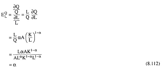
(iv) In the case of C-D production function (8.103), coefficient of partial elasticity of Q w.r.t. a change in L, K remaining constant, would be EQL = a = constant, and the coefficient of partial elasticity of Q w.r.t. a change in K, L remaining constant, would be EQL = 1 – α = constant. We may establish this property in the following way.
By definition, we have
We also have
Hence, the property (iv) is established. This property holds for the general C-D function of any degree (α + β) as given by (8.99). In that case, the elasticities would be given by α and β, respectively.
(v) For the C-D production function (8.103), the isoquants of the firm would be negatively sloped and these curves would be convex to the origin. Let us establish this property. The C-D production function is
Q = f (L,K) = ALαK1−α [(8.103)]
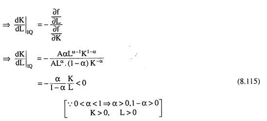
Taking total differential of (8.103), we obtain
dQ = (∂f/∂L) dL + (∂f/∂K) dK (8.114)
Now, for a movement from one point on an IQ to another (very close) point, dQ = 0 and in that case (8.114) would give us
0 = (∂f/∂L) dL + (∂f/∂K) dK
Hence, we have obtained that for the C-D function (8.103), the slope of an IQ, viz, would be negative. Again (8.115) would give us
d2K/dL2 = − α/1−α (−K/L2) = (α/1−α)(K/L2) > 0 (8.116)
It is clear from (8.116) that as L rises, the slope of the IQ, i.e., dK/dL, also rises or the absolute slope of the IQ diminishes. This implies that an IQ would be convex to the origin. This property may also be established if we use the general version of the C-D function as given by (8.100) and (8.100a), i.e., this property holds for the C-D function homogeneous of any degree, viz., a + p, a + P being not necessarily equal to 1.
(vi) For the C-D function (8.103), the expansion of the firm would be a straight line. We may establish this property in the following way.
The production function (8.103) is
Q = f (L,K) = A.Lα. K1−α
As we know, the equation of the expansion path is
Where rL = price of labour (L) = constant
And rK = price of capital (K) = constant
Since rL, rK, α = constant and the power of Land K = 1, equation (8.118) is a linear equation. The slope of this straight line is rL/rK. 1 –α/α = positive constant [... 0 < α < 1 and rL, rK > 0].
This straight line starts from the origin because when L = 0 in (8.118), we have K = 0. Therefore, for the C-D homogeneous function of degree one (8.103), the expansion path of the firm would start from the point of origin and it would be a straight line sloping upwards towards right.
In the above analysis if we use eqn. (8.100) in place of eqn. (8.103), we would obtain that for C-D production function, homogeneous of any degree, the expansion path would start from the origin and it would be a straight line sloping upward towards right, i.e., this property also holds for the general version of the C-D function, homogeneous of any degree, α + β.
(vii) For C-D production function (8.103), total output would be exhausted if the inputs L and K are paid at the rate of their respective marginal product, i.e., L. MPL + K. MPK = Q.
We may prove this in the following way.
LMPL + KMPK
= LAαLα−1K1−α + KALα (1−α) K−α
= αALαK1−α + (1−α) ALαK1−α
= ALαK1−α (α + 1 −α)
= ALαK1−α
= Q (8.119)
Hence, the property is established. This property may also be established by using the general version of the C-D function (8.100), i.e., this property holds, for C-D function homogeneous of any degree.
(viii) For C-D production function (8.103), if labour (L) and capital (K) are paid at the rate of their respective MPs, then the relative shares of labour and capital would be a and 1 – a respectively. We may prove this in the following way.
Absolute share of L in total output = LMPL
And the relative share of labour = LMPL/Q
= LAαLα−1K1−α/ALαK1−α = α (8.120)
Also, the absolute share of L in total output = KMPK
And the relative share of K = KMPK/Q
= KALα(1−αK−α)
= 1−α (8.121)
Hence, the property is established. This property may also be established by using the general C-D function (8.99) homogeneous of any degree α + β. In that case, the relative shares of labour and capital would be α and β respectively.


