Theories that Establish Relationship between Output and Investment

Here we detail about the two theories that establish relationship between output and investment.

1. The Naive Accelerator:

This hypothesis was put forwarded before the appearance of Keynes and is known as Naive because it remained unaffected by the availability of funds or size of the change in the required capital stock.

The Naive Accelerator explains that the optimum capital stock remains in fixed proportion to output shown by V in the Equation (i). It further assumed that increase in the required stock of capital can be made instantly.

K_t = VY_t …(i)

In the equation (i) K is the optimum capital stock at time t and Y_t is the current output, V is the capital output ratio which is assumed to remain constant. The Equation (i) shows that as output increases capital stock also rises by constant V. Change in the ideal stock of capital which changes due to a change in Y can be expressed in terms of change in Y i.e., the gap between the present and the past income.

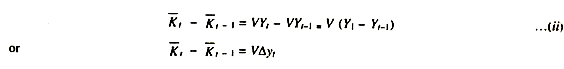
If it is assumed that optimal stock is always equal to actual stock of capital (K) then K can be replaced by K. From Equation (ii) net investment (I_n) can also be determined because the change in capital stock occurs only due to change in net investment

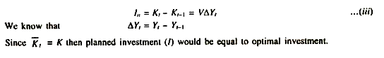
Equation (iii) shows that if net investment is to rise output (∆Y) must rise. Because if ∆Y = Nil then net investment (I_n = 0) would also be equal to zero. If we want the I_n to exist at a level (hat output must rise at a constant rate. At a time when economy is at the top of the production function i.e., maximum possible output is achieved by the economy where marginal product of inputs is zero the net investment is also zero. It is to note that gross investment will still be positive because replacement investment would be taking place in order to keep the capital stock in working condition, and the output at its maximum level. Replacement investment is a certain proportion to the capital stock.

How the capital stock rises with the increase in output Y can be shown with the help of isoquants where constant returns to scale are operating and factor prices are constant. This is shown with the help of the Fig. 18a.5.

AB, CD and LM are iso-cost lines in production. Suppose the economy is facing AB iso-cost line. It will find equilibrium level of output with minimum cost only at a point where AB line touches the highest iso-quant (Ko) which is Eq. If Y rises to Y₁ then equilibriums shows that capital stock would be raised to K₁ and then to K₁₁. Net investment and capital stock rise at constant rate as output rises at constant rate here. Keeping the minimum cost criterion, CD iso-cost line touches Y₁ isoquant at E₁.

It is assumed that capital is optimally adjusted in each time period. It is a comparative static analysis. But investment is a dynamic phenomenon. In this way naive accelerator assumes that firms are always in equilibriums, there is elastic supply of capital goods and there is no investment lags.

In the naive accelerator hypothesis it should be remembered that full capacity utilization (optimum capital stock) has been presumed. Because it is only under such situations increased level of output or demand would enhance the net investment to again rise the capital stock to its optimum level. Capital stock is raised without delay implies that it is static or comparative static study of investment. But in-fact investment is a dynamic process due to the limited resources only a part of desired capital stock can be completed.

2. The Flexible Accelerator:

According to this hypothesis wider the gap between the desired stock of capital and the existing stock of capital greater will be the rate of investment of the firm. Since, the firm cannot fill up this gap within one year for want of resources, therefore, it completes or plans to complete only a fraction (a) of the gap in each time period.

Suppose the capital stock at the end of last year was K_t-1 and the desired stock of capital at present (which depends on expected output) is K*_t The firm’s actual capital stock (K_t) at the end of current year can be calculated by the equation (i).

K, – α = (K_t* – K_t-1) …(i)

With the limited resources, the firm plans to make investment in each time period in such a way so that, at least, a fraction of the capital gap of that time period may be filled up, After rewriting the above equation we have

K_t = K_t–₁ + α (K* – K_t–₁) …(ii)

It is, therefore, clear that the net positive investment which the firm has to invest to fill up the gap between the last year’s capital stock (K _t-1,) and the capital stock at the end of the current year (K_t) would be

I_n = K_I – K _t-1 (iii)

In view of equation (i) net investment can now be written as:

I_n = α (K_t* K _t-1 ) ; where 1 > α > 0

It is self evident from the equation (iv) that wider the gap between the actual and desired capital stock the greater would be net positive investment. For instance, suppose K = 20,000 and K_t-1 = 10,000 and α = 0.5, then net investment would be

I_n = 0.5 (20,000 – 10,000) = 5,000

Net investment in the second period would become lower because of the increase in the actual stock of capital by Rs. 5,000 if the desired stock of capital in the next year remains fixed at 20,000. In this way after making investment year after year the desired stock of capital would be equal to actual stock of capital. This is called flexible accelerator where dynamic behaviour of the investment can be seen from Equation (iv) because the economic variable K_t and K_t-1 in the equation go on changing year after year.

In this way this analysis of net investment not only belongs to the current year but also belongs to the period of time for the long run. Here, the investment of one time period influences the investment of another time period. The hypothesis says that at any point of time the desired capital stock depends on the expected output. If we expect the output to fall in future years due to deflationary conditions then the desired stock of capital would fall and possibly would be less than the actual stock.

Then net investment can be negative (Reduction in replacement investment) on the other hand, if we expected output to rise in future then our desired stock of capital would be greater than the actual stock. Whether the future output rises or falls depends on the MEC. The changes in MEC (Marginal Efficiency of Capital), therefore, determines the desired stock of capital and thus the gap takes into account the future changes in output and businesses activities. Hence, Flexible Accelerator is called a study of the dynamic behaviour of investment.

Investment level also depends on the past capital stock which invariably depends on the past output. Because of this we use the term investment lag because the investment in the current year depends upon the capital stock in the past (K_t-1) or the past output.

The Dynamic Accelerator can be explained by the Cobb-Douglas Function:

I_n= α(αY/ic-K _t-1)

where α = capital part of Y

ic = investment cost.

ic, K_t-1, a and a remaining constant the net investment (I_n) has positive relationship with income (Y).

However the gap between desired stock of capital and the actual stock can be covered by increasing the actual stock through raising net investment in subsequent years as has been shown in the Fig. 18a.6.

In the Fig. 2 K_t–1 is the actual stock of capital in the past time (t – 1) and K* is the desired stock. The gap is filled by increasing net investment until time period t + 2. As the gap in subsequent years goes on decreasing net investment would also be made at decreasing rate.