Network externalities may be positive or negative. Network externalities are a special kind of externalities in which one individual’s utility for a good depends on the number of other people who consume the commodity.
In our analysis of demand we have assumed that demand for goods of different individuals are independent of one and another.
That is, demand for Pepsi by Amit depends on his own tastes, his income, price of Pepsi etc. and does not depend on Swati or Amitab Bachchan’s demand for Pepsi. The assumption of independence of demands of different individuals enabled us to derive a market demand curve for a good by simply summing up horizontally the demands of different individuals consuming a good.
However, in the real world, demand for some goods of an individual depends on other individuals’ demand for them. In such cases of interdependence of demands of different individuals economists say network externalities are present. Network externalities may be positive or negative. Network externalities are a special kind of externalities in which one individual’s utility for a good depends on the number of other people who consume the commodity.
ADVERTISEMENTS:
For example, a consumer’s demand for ‘telephone’ depends on the number of other people owning the telephone connections. People want telephone connection so that they can communicate with each other. If no one else has a telephone connection, it is certainly not useful for you to demand a telephone connection. The same applies to demand for fax machines, mobile phones, modems, internet connection etc. Internet connection is very useful to you if there are some other individuals or institutions have internet facilities with whom you can communicate.
Network externalities can arise through a fashion or stylishness. The desire or demand for wearing jeans by girls is influenced by the number of other girls who have chosen to wear them. Wearing jeans have become a fashion among the college going girls at metropolitan cities in India. To be in keeping with the fashion, more and more girls have opted for wearing jeans.
This has led to the increase in demand for jeans. However, it may be noted that network effects here go two ways. It is better if there are some others who have adopted the fashion, but if too many people go in for this, the fashion falls out of style and this adversely affects the demand for the good by others.
Another type of network externalities arises in case of complementary goods. The intrinsic value of a good is greater if its complementary good is available. Thus, it is not worthwhile to open a CD discs store in a locality if only one person in the area has a CD player. If the number of people owning CD players increases significantly, desire for opening CD (discs) store or for manufacturing CD (discs) will increase. Thus, the more the number of individuals who own CD players, the more CD (discs) will be produced.
ADVERTISEMENTS:
In this case the demand for CD players depends on the number of CD (discs) available and the demand for CD discs depends on the number of people having CD players. Thus this is a more general form of positive network externalities.
Bandwagon Effect:
The existence of positive network externalities gives rise to Bandwagon effect. Bandwagon effect refers to the desire or demand for a good by a person who wants to be in style because possession of a good is in fashion and therefore many others have it. It may be noted that this bandwagon effect is the important objective of marketing and advertising strategies of several manufacturing companies who appeal to go in for a good as people of style are buying it.
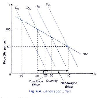
Let us explain how to derive a demand curve for a good incorporating the bandwagon effect. This is illustrated in Figure 6.4 on whose X-axis we measure the number of units of a good in question. Suppose consumers think that only 10 thousand people in Delhi have purchased the good.
This is a relatively small number of people compared to the total population of Delhi. So the other people have little incentive to buy the good to satisfy their instinct of living in style. However, some people may still purchase because it has a intrinsic value for them. In this case the demand for the good is given by the demand curve D10.
ADVERTISEMENTS:
Now suppose that they think that 20 thousand people have purchased the good. This increases the attractiveness of the good for them. As a result, they are induced to buy more of the good to keep themselves to live in fashion or style. This leads to the increase in the demand for the good which causes the demand curve for the good to shift to the right, say to D20. If the people believe that 30 thousand people have purchased the good in question, this further raises the attractiveness of the good and as a result people’s demand curve for the good further shifts to the right, say to D30.
Thus, more the number of people the consumers find have bought the good, the greater the demand for the good in question and further to the right demand curve for the good lies. This is a bandwagon effect. Thus, a bandwagon effect is an example of a positive network externality in which the quantity demanded of a good that an individual buys increases in response to the increase in the quantity purchased by other individuals.

Now, if the price of the good falls to Rs. 50, 40 thousand people buys 40 thousand units of the good and the relevant demand curve is D40. Thus, actual market demand curve DM incorporating the Bandwagon effect is obtained by joining the points on the demand curves D10, D20, D30, D40 that correspond to the quantities 10 thousand, 20 thousand, 30 thousand and 40 thousand units of the good.
It should be noted that the movement along the demand curves D10, D20, D30, and D40 individually represent how much quantity of a commodity is demanded at various prices if no bandwagon effect is operating. Thus, if price of a good falls from Rs. 100 to Rs. 50 per unit, the quantity demanded of the good will increase to 25 units of the good along a given demand curve D20 as a result of pure price effect when no bandwagon effect is working.
However, actually as a result of fall in price and resultant increase in the quantity purchased of the good by others has created a bandwagon effect and as a result at price of Rs. 50 per unit, quantity bought of the good increases to 40 thousand units.
Thus, the 15 thousand units increase in the quantity demanded is the result of bandwagon effect. It is also evident from this analysis that bandwagon effect makes the demand curve more elastic. It will be seen that demand curve DM which incorporates the bandwagon effect is more elastic than the demand curves D10, D20, D30, and D40.
Snob Effect:
In case network externalities are negative, snob effect arises. Snob effect refers to the desire to possess a unique commodity having a prestige value. Snob effect works quite contrary to the bandwagon effect. The quantity demanded of a commodity having a snob value is greater, the smaller the number of people owning its.
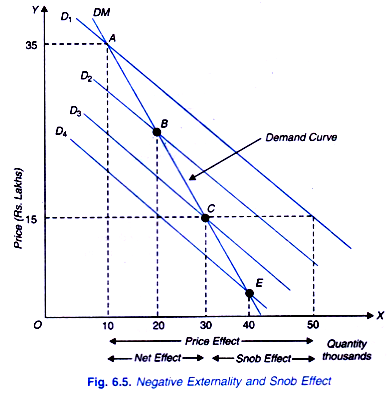
Rare works of art, specially designed sport cars, specially designed clothing made to order, very expensive luxury cars. For example, the utility one gets from a very expensive luxury car is mainly due to the prestige and status value of it which results from the fact that only few others own it. Snob effect is illustrated in Figure 6.5 where on the X-axis we measure the quantity demanded of a snob good and on the y-axis price of the good in lakhs (Rs.).
Suppose D1 is the relevant demand curve when people think that one thousand people own the commodity having a snob value. Now suppose that people think that 20 thousand people are having this good, its snob-value is lowered and as a result demand for the good decreases and demand curve shifts to the left to D2 position.
Again, if people believe that 30 thousand people happen to own the commodity, its snob value or prestige value is further reduced. As a result, desire or demand for it is further reduced and demand curve further shifts to the left. Further, if it is thought that 40 thousand people possess the good, the relevant demand curve is D4.
Thus, as a result of snob effect, the quantity demanded of the good falls as more people are believed to own it. Ultimately people come to know how many people actually own the good. If we join the points A, B, C and E which represent the quantities demanded at different number of people owning the commodity and thus incorporating snob effect we have the market demand curve DM.
It is important to note that snob effect makes the demand curve less elastic. Thus at price Rs. 35 lakhs per luxury car, its quantity demand is 10 thousands. Now, if price is reduced to Rs. 15 lakhs per luxury car, its quantity demanded would increase to 50 thousands per year, and if snob effect was not present we had moved down more along the demand curve D1. But in the presence of snob effect quantity demand increases from 10 thousand to only 30 thousand cars. Thus, in Figure 6.5 the snob effect has reduced the full effect of the fall in price so that net effect is the increase in quantity demanded from 10 thousand to 30 thousand units.
