In this essay we will discuss about Cost and Cost Curves. After reading this essay you will learn about: 1. Accounting and Economic Costs 2. Production Costs 3. Real Costs 4. Opportunity Cost 5. Private and Social Costs 6. The Cost Function 7. The Traditional Theory of Costs 8. The Modern Theory of Costs.
Contents:
- Essay on Accounting and Economic Costs
- Essay on Production Costs
- Essay on Real Costs
- Essay on Opportunity Costs
- Essay on Private and Social Costs
- Essay on the Cost Function
- Essay on the Traditional Theory of Costs
- Essay on the Modern Theory of Costs
Essay # 1. Accounting and Economic Costs:
Money (accounting or explicit) costs are the total money expenses incurred by a firm in producing a commodity.
They include wages and salaries of labour; cost of raw materials; expenditures on machines and equipment; depreciation and obsolescence charges on machines; building and other capital goods; rent on buildings; interest on capital borrowed; expenses on power, light, fuel, advertisement and transportation; insurance charges and all types of taxes.
ADVERTISEMENTS:
There are the accounting costs which an entrepreneur takes into consideration in making payments to the various factors of production. These money costs are also known as explicit costs that an accountant records in the firm’s books.
“Explicit costs are the payments to outside suppliers of inputs.” There are other types of economic costs called implicit costs. Implicit costs are the imputed value of the entrepreneur’s own resources and services. According to Salvatore, “Implicit costs are the value of owned inputs used by the firm in its own production process.”
The salary of the owner-manager who is content with having normal profits but does not receive any salary; estimated rent of the building if it belongs to the entrepreneur, and interest on capital invested by the entrepreneur himself at the market rate of interest. Thus economic costs include accounting costs plus implicit costs, that is, both explicit and implicit costs.
Essay # 2. Production Costs:
In the production process, many fixed and variable factors (inputs) are used. They are employed at various prices. The expenditures incurred on them are the total costs of production of a firm. Such costs are divided into total variable costs and total fixed costs.
ADVERTISEMENTS:
Total variable costs are those expenses of production which change with the change in the firm’s output. Larger outputs require larger inputs of labour, raw materials, power, fuel, etc. which increase the expenses of production.
When output is reduced, variable costs also diminish. They cease when production stops altogether. Marshall called these variable costs as prime costs of production. Total fixed costs, called supplementary costs by Marshall, are those expenses of production which do not change with the change in output.
They are rent and interest payments, depreciation charges, wages and salaries of the permanent staff, etc. Fixed costs have to be incurred by the firm, even if it stops production temporarily. Since these costs are over and above the usual expenses of production, they are described as overhead costs in business parlance.
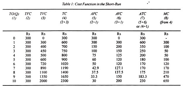
The relation between total costs, variable costs and fixed costs is presented in Table 1 where column (1) indicates different levels of output from 0 to 10 units. Column (2) indicates that total fixed costs (TFC) remain at Rs.300 at all levels of output. Column (3) shows total variable costs (TVC) which are zero when output is nothing and they continue to increase with the rise in output.
ADVERTISEMENTS:
In the beginning, they rise quickly, and then they slow down as the firm enjoys economies of large scale production with further increases in output and later on, due to diseconomies of production, the variable costs start rising rapidly. Column (4) relates to total costs (TC) which are the sum of columns (2), and (3) i.e., TC = TFC + TVC. Total costs vary with total variable costs when the firm starts production.
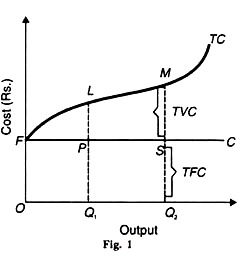
The cost relations are shown in Figure 1 where the distance between the horizontal line FC and X axis measures the total fixed costs, and the total variable costs is the distance above the FC curve, i.e., in between TC and TFC. Thus at OQ1 level of output, TC = TFC + TVC is Q1L = Q1P + PL. Similarly, at OQ, level of output, Q2M = Q2S + SM.
Its importance:
This distinction between fixed costs and variable costs is valid only during the short period. In the short run, a firm may be selling its products at a loss but it will continue able, for the firm is in a position to change its fixed plant, equipment, the amount of labour, etc. Thus all costs become variable in the long-run and the firm must cover them at the ruling price otherwise it will cease to exist.
Essay # 3. Real Costs:
Money costs are the expenses of production from the point of view of the producer. But they tell us nothing about what lies behind these costs. Marshall thought that the efforts and sacrifices undergone by the various members of the society in producing a commodity are the real costs of production.
The efforts and sacrifices made by the capitalist to save and invest, by the workers in foregoing leisure, and by the landlords in the use of land, all constitute real costs. But real costs seldom equal monetary expenses of production.
Work which is disagreeable and unpleasant does not carry high wages and a light job low wages. Neither can the sacrifice of a person who saves Rs.50 be equated to the painful efforts of a worker receiving Rs.50 as wages. Thus the money costs and the real costs of production do not correspond with each other in the short or the long-run.
Essay # 4. Opportunity Cost:
Since resources are scarce, they cannot be used to produce all things simultaneously. Therefore, if they are used to produce one thing, they have to the withdrawn from other uses. Thus the cost of the one is the alternative forgone. It is the opportunity missed or alternative forgone in having one thing rather than the other or in putting a factor-service to one use instead of the other.
ADVERTISEMENTS:
In the words of Benham, “The opportunity cost of anything is the next best alternative that could be produced instead by the same factors or by an equivalent group of factors, costing the same amount of money.” The cost of using land for wheat growing is the value of alternative crop that could have been grown on it.
The real cost of labour is what it could get in some alternative employment. The cost of capital to the capitalist is the amount of interest he could earn elsewhere. The normal earnings of management are what an entrepreneur could earn as a manager in some other joint stock company. In this way, opportunity cost is the cost of the opportunity missed or alternative forgone.
Opportunity cost includes both explicit and implicit costs. Explicit costs are those expenses which are incurred by the firm in buying the goods and services directly. They include wages and salaries, payments for raw materials, power, light, fuel, advertisement, transportation, and taxes. Implicit costs are the imputed value of the entrepreneur’s own resources and services.
ADVERTISEMENTS:
In other words, implicit costs are what self-employed and self-owned resources could have earned in their best alternative uses. Thus implicit wages, implicit rent and implicit interest refer to the highest wage, rent and interest which the entrepreneur could have received for his labour, building and capital, had he loaned them to others instead of using them himself.
But this does not mean that only implicit costs are included in opportunity cost and explicit costs are excluded from it. In fact, the opportunity cost of any firm includes all alternatives forgone whether they are explicit or implicit.
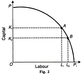
The concept of opportunity cost is explained diagrammatically in Figure 2 with the help of the production possibility curve PP1. At combination A on this curve, the producer uses OL1 of labour and OK1 of capital. If he wants to use L1L2 more labour, he will have to forgo K1K2 of capital. Thus the opportunity cost of L1L2 labour is K1K2 of capital.
ADVERTISEMENTS:
Importance:
The concept of opportunity cost has wide application to economic problems:
1. It is applicable to the determination of factor prices and in international trade.
2. It can also be applied to consumption and public expenditure. The cost of seeing a movie is the pen whose purchase is forgone by a student. For the society, the cost of setting up an ammunition factory is the civilian benefits which are sacrificed.
3. It is the opportunity cost which explains the phenomenon of price. Since there is scarcity of goods and factor services, they are put to alternative uses and thus command a price. If they were in plenty, there would be no alternatives forgone, no opportunity cost and no price. They are priced because of their opportunity cost.
It’s Limitations:
ADVERTISEMENTS:
However, the concept of opportunity cost is not free from certain limitations.
1. It is not applicable to those factor services which are fixed, for a fixed or specific factor has no alternatives and hence its opportunity cost is nil.
2. If factors are prevented from moving or are themselves reluctant to move to alternative occupations, then their prices do not reflect opportunity cost.
3. There may be a difference between individual and social costs. A smoky factory in the heart of the town may involve large sacrifice of alternatives in the form of hazards to health which cannot be measured in money terms.
4. The forgone alternatives are often not clearly ascertainable. If the alternatives are easily ascertainable there is no problem at all. But if the factor is lumpy as in the modern complex productive system, it has no alternative use once it is installed. Durable capital equipment has no opportunity cost. But its cost does enter into the price of the product which it helps to produce.
5. It is based on the assumption of perfect competition which is not found in reality.
Essay # 5. Private and Social Costs:
The terms private and social costs were first used by Pigou in his The Economics of Welfare (1932). Private costs are the costs incurred by a firm in producing a commodity or service. These include both explicit and implicit costs.
ADVERTISEMENTS:
However, the production activities of a firm may lead to economic benefit or harm for others. For example, production of commodities like steel, rubber and chemicals, pollutes the environment which leads to social costs.
On the other hand, production of such services as education, sanitation services, park facilities, etc. leads to social benefits. Take for instance, education which not only provides higher incomes and other satisfactions to the recipients but also more enlightened citizens to the society.
If we add together the private costs of production and economic damage upon others such as environmental pollution, etc., we arrive at social costs.
Essay # 6. The Cost Function:
The cost function expresses a functional relationship between total cost and factors that determine it. Usually, the factors that determine total cost of production (C) of a firm are the output (Q), the level of technology (T), the prices of factors (Pf) and the fixed factors (F).
Symbolically, the cost function becomes:
ADVERTISEMENTS:
C = f (Q, T, Pf, F)
Such a comprehensive cost function requires multi-dimensional diagrams which are difficult to draw.
Assumptions:
In order to simplify the cost analysis, certain assumptions are made.
1. It is assumed that a firm produces a single homogeneous good (q) with the help of certain factors of production.
2. Some of these factors are employed in fixed quantities, whatever the level of output of the firm in the short run. So they are assumed to be given.
ADVERTISEMENTS:
3. The remaining factors are variable whose supply is assumed to be known and available at fixed market prices.
4. The technology which is used for the production of the good is assumed to be known and fixed.
5. It is assumed that the firm adjusts the employment of variable factors in such a manner that a given output Q of the good q is obtained at the minimum total cost, C.
Thus the total cost function is expressed as:
С = f (Q)
which means that the total cost (C) is a function (f) of output (Q), assuming all other factors as constant. The cost function is observed both in the short-run and the long-run. The short-run costs are those costs of production at which the firm operates in one given period when one or more factors of production are fixed in quantity.
Therefore, the firm has some fixed costs and some variable costs. On the other hand, “the long-run costs are planning costs or ex ante costs, in that they present the optimal possibilities for expansion of the output and thus help the entrepreneur to plan his future activities.”
In the long-run, there are no fixed factors of production and hence no fixed costs. In the long-run, all factors being variable, all costs are also variable. Therefore, the firm plans for the future, given its fixed capital equipment. But it operates on the short- run cost curves relating to each plant.
Essay # 7. The Traditional Theory of Costs:
The traditional theory of costs analyses the behaviour of cost curves in the short- run and long-run and arrives at the conclusion that both the short-run and long-run cost curves are U-shaped but the long-run cost curves are flatter than the short-run cost curves.
(A) Firm’s Short-Run Cost Curves:
The short run is a period in which the firm cannot change its plant, equipment and the scale of organisation. To meet the increased demand, it can raise output by hiring more labour and raw materials or asking the existing labour force to work overtime.
The scale of organisation being fixed, the short-run total costs (TC) are divided into total fixed costs (TFC) and total variable costs (TVC):
TC = TFC + TVC
Total Costs are the total expenses incurred by a firm in producing a given quantity or a commodity. They include payments for rent, interest, wages, taxes and expenses on raw materials, electricity, water, advertising, etc.
Total Fixed Costs are those costs of production that do not change with output. They are independent of the level of output. In fact, they have to be incurred even when the firm stops production temporarily. They include payments for renting land and buildings, interest on borrowed money, insurance charges, property tax, depreciation, maintenance expenditures, wages and salaries of the permanent staff, etc.,
They are also called overhead costs. Total Variable Costs are those costs of production that change directly with output. They rise when output increases, and fall when output declines. They include expenses on raw materials, power, water, taxes, hiring of labour, advertising, etc. They are also known as direct costs.
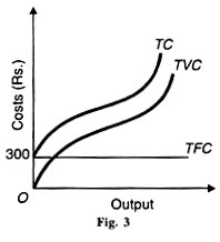
The curves relating to these three total costs are shown diagrammatically in Figure 3. The TC curve is a continuous curve which shows that with increasing output total costs also increase. This curve cuts the vertical axis at a point above the origin and rises continuously from left to right.
This is because even when no output is produced, the firm has to incur fixed costs. The TFC curve is shown as parallel to the output axis because total fixed costs (Rs.300) are the same whatever the level of output.
The TVC curve has an inverted-S shape and starts from the origin О because when output is zero, the TVCs are also zero (Table 30.1). They increase as output increases. So long as the firm is using less variable factors in proportion to the fixed factors, the total variable costs rise at a diminishing rate.
But after a point, with the use of more variable factors in proportion to the fixed factors, they rise steeply because of the application of the law of variable proportions. Since the TFC curve is a horizontal straight line, the TC curve follows the TVC curve at an equal vertical distance.
Short-Run Average Costs. In the short run analysis of the firm, average costs are more important than total costs. The units of output that a firm produces do not cost the same amount to the firm. But they must be sold at the same price. Therefore, the firm must know the per-unit cost or the average cost. The short-run average costs of a firm are the average fixed costs, the average variable costs, and average total costs.
Average Fixed Costs (or AFC) equal total fixed costs at each level of output divided by the number of units produced:
AFC = TFC/Q
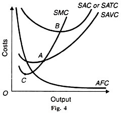
The average fixed costs diminish continuously as output increases. This is natural because when a constant figure, total fixed costs are divided by a continuously increasing unit of output, the result is continuously diminishing average fixed costs. Thus the AFC curve is a downward sloping curve which approaches the quantity axis without touching it, as shown in Figure 4. It is a rectangular hyperbola.
Short-Run Average Variable Costs (or SAVC) equal total variable costs at each level of output divided by the number of units produced:
SAVC = TVC/Q
The average variable costs decline with the rise in output as larger quantities of variable factors are applied to fixed plant and equipment. But eventually they begin to rise due to the law of diminishing returns. Thus the SAVC curve is U-shaped, as shown in Figure 4.
Short-Run Average Total Costs (or SATC or SAC) are the average costs of producing any given output.
They are arrived at by dividing the total costs at each level of output by the number of units produced:
SAC or SATC = TC/Q = TFC/Q + TVC/Q = AFC + AVC
U-shape of SAC curve:
Average total costs reflect the influence of both the average fixed costs and average variable costs. At first, average total costs are high at low levels of output because both average fixed costs and average variable costs are large. But as output increases, the average total costs fall sharply because of the steady decline of both average fixed costs and average variable costs till they reach the minimum point.
This results from the internal economies, from better utilisation of existing plant, labour, etc. The minimum point В in the figure represents optimal capacity.
As production is increased after this point, the average total costs rise quickly because the fall in average fixed costs is negligible in relation to the rising average variable costs. The rising portion of the SAC curve results from producing above capacity and the appearance of internal diseconomies of management, labour, etc. Thus the SAC curve is U-shaped, as shown in Figure 4.
The U-shape of the SAC curve can also be explained in terms of the law of variable proportions. This law tells that when the quantity of one variable factor is changed while keeping the quantities of other factors fixed, the total output increases but after some time it starts declining.
Machines, equipment and scale of production are the fixed factors of a firm that do not change in the short-run. On the other hand, factors like labour and raw materials are variable. When increasing quantities of variable factors are applied on the fixed factors, the law of variable proportions operates.
When, say the quantities of a variable factor like labour are increased in equal quantities, production rises till fixed factors like machines, equipment, etc., are used to their maximum capacity. In this stage, the average costs of the firm continue to fall as output increases because it operates under increasing returns.
Due to the operation of the law of increasing returns, when the variable factors are increased further, the firm is able to work the machines to their optimum capacity.
It produces the optimum output and its average costs of production will be the minimum which is revealed by the minimum point of the SAC curve, point В in Figure 30.4. If the firm tries to raise output after this point by increasing the quantities of the variable factors, the fixed factors like machines would be worked beyond their capacity.
This would lead to diminishing returns. The average costs will start rising rapidly. Hence due to the working of the law of variable proportions, the short-run AC curve is U-shaped.
Short-run Marginal Cost. A fundamental concept for the determination of the exact level of output of a firm is the marginal cost.
Marginal cost is the addition to total cost by producing an additional unit of output:
SMC = ∆TC/∆Q
Algebraically, it is the total cost of n – 1 unit minus the total cost of n-1 units of output, MCn = TCn – TCn-1. Since total fixed costs do not change with output, therefore, marginal fixed cost is zero.
So marginal cost can be calculated either from total variable costs or total costs. The result would be the same in both the cases. As total variable costs or total costs first fall and then rise, marginal cost also behaves in the same way. The SMC curve is also U-shaped, as shown in Figure 4. It first falls and is below the SAC curve and then starts rising from point C, passes through the minimum point В of the SAC curve and moves above it.
Relationships of Short-Run Cost Curves:
The relationships of short-run cost curves are explained in terms of Figure 4.
(a) The AFC curve declines continuously and is asymptotic to both axes. It means that the AFC curve approaches both axes but never touches either X-axis or Y-axis. Thus the AFC curve is a rectangular hyperbola.
(b) The SAVC curve first declines, reaches a minimum at point A, and rises thereafter. When the SAVC curve reaches its minimum point A, the SMC curve equals the SAVC curve.
(c) The SAC curve first declines, reaches a minimum at point B, and rises thereafter. When the SAC curve reaches its minimum point B, the SMC curve equals the SAC curve. Since SAC = AFC + AVC, the vertical distance between the SAC and the SAVC curves gives the AFC curve, So there is no need to draw a separate AFC curve. As output expands, the vertical distance between the SAC curve and the SAVC curve declines because of the falling AFC curve.
(d) Relation between AC and MC Curves:
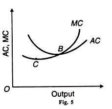
There is a direct relationship between AC and MC curves as shown in Figure 5. Both the AC curve and the MC curve are U-shaped.
1. When AC falls, MC is less than AC. This is because the fall in MC is related to one unit of output while in the case of AC the same decline is spread over all units of output. That is why the fall in AC is less and that in MC is more. This also explains the fact that MC reaches its minimum point С before the minimum point В of AC is reached. So When MC starts rising, AC is still declining.
2. When AC is minimum, MC equals AC. The MC curve cuts the AC curve from below at its minimum point B in the figure.
3. When AC rises, MC is greater than AC. MC is above AC when AC is rising but the rise in MC is greater than AC. This is because the rise in MC is the result of the increase in one unit of output while in the case of AC the same increase is spread over all units of output.
4. Nothing can be said about the direction of MC, when AC rises or falls. When AC is falling, it is not essential that MC must fall. MC can increase or fall but it is definite that MC will he less than AC. Similarly, when AC is increasing, it is not essential that MC must rise. MC can fall or rise but it is definite that MC will be larger than AC. But if AC is constant, MC must be constant.
5. Relation between AC and MC is the same in the short-run and the long- run. But their shapes differ: both are U-shaped in the short- run and flat in the long-run.
(e) Relation between SMC and SAVC Curves:
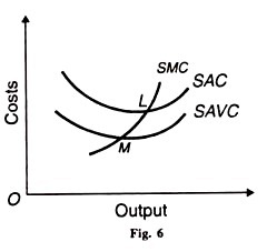
The SMC curve bears a close relationship to the SAVC curve along with the SAC curve. So long as the SMC curve lies below the SAVC and SAC curves, it continues to fall and its rate of fall is greater than that of SAC and SAVC curves. But the SAVC and SAC curves start rising from the points M and L respectively where the SMC curve touches them, as shown in Figure 6.
The SMC curve passes O through the minimum point M of the SAVC curve to the left of the minimum point L of the SAC curve. Since AC is the sum total of SAVC + AFC, therefore when SAVC is at its minimum point, AFC is falling and it takes time for SAC to reach its minimum point.
M and L are thus the respective minimum points of the SAVC and SAC curves. After O these points, the SMC curve rises sharply and is above the SAVC and SAC curves.
Conclusion:
Thus the short-run cost curves of a firm are the SAVC curve, the AFC curve, the SAC curve and the SMC curve. Out of these four curves, the AFC curve is insignificant for the determination of the firm’s exact output and is, therefore, generally neglected.
(B) Firm’s Long-Run Cost Curves:
In the long-run, there are no fixed factors of production and hence no fixed costs. The firm can change its size or scale of plant and employ more or less inputs. Thus in the long- run, all factors are variable and hence all costs are variable.
The long-run average total cost (or LAC) curve of the firm shows the minimum average cost of producing various levels of output from all possible short-run average cost curves (SAC). Thus the LAC curve is derived from the SAC curves.
The LAC curve can be viewed as a series of alternative short-run situations into any one of which the firm can move. Each SAC curve represents a plant of a particular size which is suitable for a particular range of output.
The firm will, therefore, make use of the various plants up to that level where the short-run average costs fall with increase in output. It will not produce beyond the minimum short-run average cost of producing various outputs from all the plants used together.
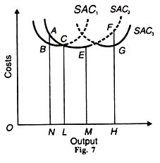
Let there be three plants represented by their short-run average cost curves SAC1 SAC2 and SAC3 in Figure 7. Each curve represents the scale of the firm. SAC: depicts a lower scale while the movement from SAС3 to SAC3 shows the firm to be of a larger size. Given this scale of the firm, it will produce up to the least cost per unit of output.
For producing ON output, the firm can use SAC1 or SAC2 plant. The firm will, however, use the scale of plant represented by SAC1, since the average cost of producing ON output is NB which is less than NA, the cost of producing this output on SAC2 plant.
If the firm is to produce OL output, it can produce at either of the two plants. But it would be advantageous for the firm to use the plant SAC2 for the OL level of output. But it would be more profitable for the firm to produce the larger output OM at the lowest average cost ME from this plant.
However, for output OH, the firm would use the SAC3 plant where the average cost HG is lower than HF of the SAC2 plant. Thus in the long-run, in order to produce any level of output, the firm will use that plant which has the minimum unit cost.
If the firm expands its scale by the three stages represented by SAC1 SAC2 and SAC3 curves, the thick wave-like portions of these curves form the long-run average cost curve. The dotted В portions of these SAC curves are of no consideration during the о long-run because the firm would change the scale of plant rather than operate on them.
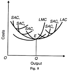
But the average long-run cost curve LAC is usually shown as a smooth curve fitted to the SAC curves so that it is tangent to each of them at some point, as shown in Figure 8 where SAC1 SAC2, SAC3, SAC4 and SAC5 are the short-run cost curves. It is tangent to all the SAC curves but only to one at its minimum point. The LAC is tangent to the lowest point E of the curve SAC3 in Figure 8 at OQ optimum output.
The plant SAC3 which produces this OQ optimum output at the minimum cost QE is the optimum plant, and the firm producing this optimum output at the minimum cost with this optimum plant is the optimum firm. If the firm produces less than the optimum output OQ, it is not working its plant to full capacity and if it produces beyond OQ, it is overworking its plants.
In both the cases, the plants SAC2 and SAC.4 have higher average costs of production than the plant SAC3.
The LAC curve is known as an “envelope” curve because it envelopes all the SAC curves. According to Stonier and Hague, “In a sense, the term ‘envelope’ is misleading. An envelope is physically distinct from the letter which it contains.
But every point on an envelope long-run cost curve is also a point on one of the short- run cost curves which it envelopes.” According to Prof. Chamberlin: “It is composed of plant curves; it is the plant curve. But it is better to call it a “planning” curve because the firm plans to expand its scale of production over the long-run.”
The long-run marginal cost (LMC) curve of the firm intersects SAC3 and LAC curves at the minimum point E where the SMC curve will also pass through. The SMC curve has not been shown in the figure to avoid confusion.
Why is LAC Curve Flatter than SAC Curve?
Though the LAC curve is U-shaped, yet it is flatter than the short-run average cost (SAC) curve. It means that the LAC curve first falls slowly and then rises gradually after a minimum point is reached.
Initially, the LAC curve gradually slopes downwards due to the availability of certain economies of scale like the economical use of indivisible factors, increased specialisation and the use of technologically more efficient machines or factors.
1. Indivisibility of Factors:
The returns to scale increase because of the indivisibility of factors of production. When a business unit expands, the returns to scale increase because the indivisible factors are employed to their maximum capacity.
2. Specialisation and Division of Labour:
When the scale of the firm is expanded, there is wide scope for specialisation of labour and equipment. Work can be divided into small tasks and workers can be concentrated on narrower range of processes. For this, specialised equipment can be installed. Thus with specialisation, efficiency increases and increasing returns to scale follow.
3. Internal Economies:
As the firm expands, it enjoys internal economies of production. It may be able to install better machines, sell its products more easily, borrow money cheaply, procure the services of more efficient manager and workers, etc. All these economies help in increasing the returns to scale more than proportionately.
4. Economics and Diseconomies Balance:
After the minimum point of the long-run average cost is reached, the LAC curve may flatten out over a certain range of output with the expansion of the scale of production. In such a situation, the economies and diseconomies balance each other and the LAC curve has a disc base.
5. Diseconomies:
With further expansion of scale, the diseconomies like the difficulties of coordination, management, labour and transport arise which more than counterbalance the economies so that the LAC curve begins to rise. As the industry continues to expand the demand for skilled labour, land, capital, etc. rises.
Transport and marketing difficulties also emerge. Prices of raw materials go up. All these factors lead to diminishing returns to scale and tend to raise costs.
Conclusion:
In either case, the LAC curve falls or rises more slowly than the SAC curve because in the long-run all costs become variable and few are fixed. The plant and equipment can be worked fully and more efficiently so that both the average fixed costs and the average variable costs are lower in the long-run than in the short-run. That is why the LAC curve is flatter than the SAC curve.
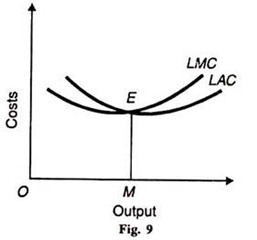
Similarly, the LMC curve is flatter than SMC curve, because all costs are variable and there are few fixed costs. In the short-run, the market cost is related to both the fixed and variable costs. As a result, the SMC curve falls and rises more swiftly than the LMC curve.
The LMC curve bears the usual relation to the LAC curve. It first falls and is below the LAC curve. Then it rises and cuts the LAC curve at its lowest point E and is above the latter throughout its length, as shown in Figure 9.
Essay # 8. The Modern Theory of Costs:
The modern theory of costs differs from the traditional theory of costs with regard to the shapes of the cost curves. In the traditional theory, the costs curves are U-shaped. But in the modern theory which is based on empirical evidences, the short-run SAVC curve and the SMC curve coincide with each other and are a horizontal straight line over a wide range of output.
So far as the LAC and LMC curves are concerned, they are L-shaped rather than U-shaped. We discuss below the nature of short-run and long-run cost curves according to the modern theory.
(1) Short-Run Cost Curves:
As in the traditional theory, the short-run cost curves in the modern theory of costs are the AFC, SAVC, SAC and SMC curves. As usual, they are derived from the total costs which are divided into total fixed costs and total variable costs. But in the modern theory, the SAVC and SMC curves have a saucer-type shape or bowl-shape rather than a U-shape.
As о the AFC curve is a rectangular hyperbola, the SAC curve has a U-shape even in the modern version. Economists have investigated this behaviour pattern of the short-run cost curves on the basis of empirical studies. According to them, a modern firm chooses such a plant which it can operate easily with the available variable direct factors.
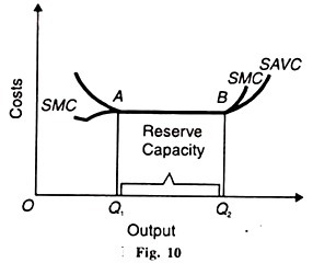
Such a plant possesses some reserve capacity and much flexibility. The firm installs this type of plant in order to produce the maximum rate of output over a wide range to meet any increase in demand for its product. The saucer shaped SAVC and SMC curves are shown in Figure 10. To begin with, both the curves first fall up to point A and the SMC curve lies below the SAVC curve.
The falling part of the SAVC shows the reduction in costs due to the better utilisation of the fixed factor and the consequent increase in skills and productivity of the variable factor (labour). With better skills, the wastes in raw materials are also being reduced and a better utilisation of the whole plant is reached.
So far as the flat stretch of the saucer-shaped SAVC curve over Q1Q2 range of output is concerned, the empirical evidence reveals that the operation of a plant within this wide range exhibits constant returns to scale and the SAVC curve is saucer-shaped.
The reason for the saucer-shaped SAVC curve is that the fixed factor is divisible. The SAV costs are constant over a large range up to the point at which the entire fixed factor is used. Moreover, the firm’s SAV costs tend to be constant over a wide range of output because there is no need to depart from the optimal combination of labour and capital in those plants that are kept in operation.
Thus there is a large range of output over which the SAVC curve will be flat. Over that range SMC and SAVC are equal and are constant per unit of output. The firm will, therefore, continue to produce within Q1Q2 reserve capacity of the plant.
After point B, both the SAVC and SMC curves start rising. When the firm departs from its normal or the load factor of the plant in order to obtain higher rates of output beyond Q2 it leads to higher SAVC and SMC.
The increase in costs may be due to the overtime operations of the old and less efficient plant leading to frequent breakdowns, wastage of raw materials, reduction in labour productivity and increase in labour cost due to overtime operations. In the rising portion of the SAVC curve beyond point B, the SMC curve lies above it.
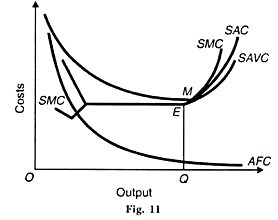
The short-run average total cost curve (SATC or SAC) is obtained by adding vertically the average fixed cost curve (AFC) and the SAVC curve at each level of output. The SAC curve, as shown in Figure 11 continues to fall till the Q reserve capacity of the plant is fully exhausted.
Beyond that output level, the SAC curve rises as output increases. The smooth and continuous fall in the SAC curve up to the Q level of output is due to the fact that the AFC curve is a rectangular hyperbola and the SAVC curve first falls and then becomes horizontal within the range of reserve capacity.
Beyond the Q output-level, it starts rising steeply. But the minimum point M of the SAC curve where the SMC curve intersects it, is to the right of point E of the SAVC curve. This is because the SAVC curve starts rising steeply from point E while the AFC curve is falling at a very low rate.
(2) Long-Run Cost Curves:
Empirical evidence about the long-run average cost curve reveals that the LAC curve is L-shaped rather than U-shaped. In the beginning, the LAC curve rapidly falls but after a point “the curve remains flat, or may slope gently downwards, at its right-hand end.” Economists have assigned the following reasons for the L- shape of the LAC curve.
1. Production and Managerial Costs:
In the long run, all costs being variable, production costs and managerial costs of a firm are taken into account when considering the effect of expansion of output on average costs. As output increases, production costs fall continuously while managerial costs may rise at very large scales of output.
But the fall in production costs outweighs the increase in managerial costs so that the LAC curve falls with increases in output. We analyse the behaviour of production and managerial costs in explaining the L-shape of the LAC curve.
(i) Production Costs:
As a firm increases its scale of production, its production costs fall steeply in the beginning and then gradually. This is due to the technical economies of large scale production enjoyed by the firm. Initially, these economies are substantial. But after a certain level of output when all or most of these economies have been achieved, the firm reaches the minimum optimal scale or minimum efficient scale (MES).
Given the technology of the industry, the firm can continue to enjoy some technical economies at outputs larger than the MES for the following reasons:
(a) From further decentralisation and improvement in skills and productivity of labour;
(b) From lower repair costs after the firm reaches a certain size; and
(c) By itself producing some of the materials and equipment cheaply which the firm needs instead have buying them from other firms.
(ii) Managerial Costs:
In modern firms, for each plant there is a corresponding managerial set-up for its smooth operation. There are various levels of management, each having a separate management technique applicable to a certain range of output. Thus, given a managerial set-up for a plant, its managerial costs first fall with the expansion of output and it is only at a very large scale of output, they rise very slowly.
To sum up, production costs fall smoothly and managerial costs rise slowly at very large scales of output. But the fall in production costs more than offsets the rise in managerial costs so that the LAC curve falls smoothly or becomes flat at very large scales of output, thereby giving rise to the L-shape of the LAC curve.
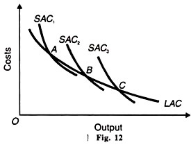
In order to draw such an LAC curve, we take three short-run average cost curves SAC1 SAC2, and SAC3 representing three plants with the same technology in Figure 12. Each SAC curve includes production costs, managerial costs, other fixed costs and a margin for normal profits. Each scale of plant (SAC) is subject to a typical load factor capacity so that points A, В and С represent the minimal optimal scale of output of each plant.
By joining all such points as A, В and С of a large number of SACs, we trace out a smooth and continuous LAC curve, as shown in Figure 13. This curve does not turn up at very large scales of output. It does not envelope the SAC curves but intersects them at the optimal level of output of each plant.
2. Technical Progress:
Another reason for the existence of the L-shaped LAC curve in the modern theory of costs is technical progress. The traditional theory of costs assumes no technical progress while explaining the U-shaped LAC curve. The empirical results on long-run costs conform the widespread existence of economies of scale due to technical progress in firms.
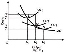
The period, between which technical progress has taken place, the long- run average costs show a falling trend. The evidence on diseconomies is much less certain. So an upturn of the LAC at the top end of the size scale has not been observed. The L-shape of the LAC curve due to technical progress is explained in Figure 13.
Suppose the firm is producing OQ1 output on LAC1 curve at a per unit cost of ОС1 output on LAC1 curve at a per unit cost of OC1 If there is an increase in demand for the firm’s product to OQ2 with no change in technology, the firm will produce OQ2 output along the LAC1 curve at a per unit cost of ОС’.
If, however, there is technical progress in the firm, it will install a new plant having LAC2 as the long- run average cost curve. On this plant, it produces OQ2 output at a lower cost OC2 per unit.
Similarly, if the firm decides to increase its output to OQ3 to meet further rise in demand, technical progress may have advanced to such a level that it installs the plant with the LAC3 curve. Now it produces OQ3 output at a still lower cost OC3 per unit.
If the minimum points, L, M and N of these U-shaped long-run average cost curves LAC1 LAC2 and LAC3 are joined by a line, it forms an L-shaped gently sloping downward curve LAC.
3. Learning:
Another reason for the L-shaped long-run average cost curve is the learning process. Learning is the product of experience. If experience in this context can be measured by the amount of a commodity produced, then higher the production is, the lower is per unit cost. The consequences of learning are similar to increasing returns.
First, the knowledge gained from working on a large scale cannot be forgotten.
Second, learning increases the rate of productivity.
Third, experience is measured by the aggregate output produced since the firm first started to produce the product.
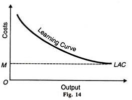
“Learning by doing” has been observed when firms start producing new products. After they have produced the first unit, they are able to reduce the time required for production and thus reduce their per unit cost. Figure 14 shows a learning curve LAC which relates the cost of producing a given output to the total output over the entire time period.
Growing experience with making the product leads to falling costs as more and more of it is produced. When the firm has exploited all learning possibilities, costs reach a minimum level, M in the figure. Thus the LAC curve is L-shaped due to learning by doing.
Relation between LAC and LMC Curves:
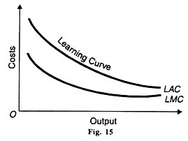
In the modern theory of costs, if the LAC curve falls smoothly and continuously even at very large scales of output, the LMC curve will lie below the LAC curve throughout its length, as shown in Figure 15.
If the LAC curve is downward sloping up to the point of a minimum optimal scale of plant or a minimum efficient scale (MES) of plant beyond which no further scale economies exist, the LAC curve becomes horizontal. In this case, the LMC curve lies below the LAC curve until the MES point M is reached, and beyond this point the LMC curve coincides with the LAC curve, as shown in Figure 16.
Conclusion:
The majority of empirical cost studies suggest that the U-shaped cost curves postulated by the traditional theory are not observed in the real world. Two major results emerge predominantly from most studies.
First, the SAVC and SMC curves are constant over a wide-range of output.
Second, the LAC curve falls sharply over low levels of output, and subsequently remains practically constant as the scale of output increases. This means that the LAC curve is L-shaped rather than U-shaped. Only in very few cases diseconomies of scale were observed, and these at very high levels of output.

