
In this essay we will discuss about Supply of a Commodity. After reading this essay you will learn about: 1. Meaning of Supply 2. The Law of Supply 3. The Elasticity of Supply 4. The Short-Run Supply Curve of the Firm and Industry 5. The Long-Run Supply Curve of the Firm and Industry 6. Supply Curve under Monopoly or Imperfect Competition.
Contents:
- Essay on the Meaning of Supply
- Essay on the Law of Supply
- Essay on the Elasticity of Supply
- Essay on the Short-Run Supply Curve of the Firm and Industry
- Essay on the Long-Run Supply Curve of the Firm and Industry
- Essay on the Supply Curve under Monopoly or Imperfect Competition
Essay # 1. Meaning of Supply:
By supply is meant the quantities of a commodity or service which a seller is willing and able to offer for sale at various prices during a given period of time. Thus supply is always at a price and in relation to a period of time. The higher the price, The greater will be the quantity of a commodity that will be supplied by a producer, and vice versa. Therefore, the relation between price and quantity supplied is direct and positive.
Factors Influencing Supply:
ADVERTISEMENTS:
The quantity supplied of a commodity is not dependent upon its price alone but on a number of factors such as the prices of other commodities, the price of factors used in its production, the goals of producers and the state of technology, these factors can better written in the form of an equation known as the supply function thus:
S0 = f (PQ: Pa Pb,……………..;F1, F2……….;G; T)
Where S is the supply of commodity Q which is a function f of the price of commodity PQ, of prices of other commodities Pa, Pb, etc., of prices of factors of production F1 F2, etc.; of the goals of producers G; and of the state of technology T.
We discuss these determinants of supply below:
ADVERTISEMENTS:
1. Price of the Commodity:
The higher the price of a commodity, the larger will be the quantity supplied, and vice versa.
2. Price of other Commodities:
A change in the price of another commodity also affects the supply of a commodity. For instance, if the price of good A rises, the producer of good В may produce less of good В and switch over to the production of good A in order to sell more of it.
ADVERTISEMENTS:
3. Prices of Factors used in its Production:
If the price of any one factor of production (i.e. labour or capital) used in the production of a commodity increases, its cost of production and price will increase. As a result, its output will fall and the supply will be reduced. The reverse will happen in the case of a fall in the price of a factor.
4. Goals of Producers:
If a producer aims at maximising profit, he will produce less of the commodity which involves large risk. A producer who aims at maximising his sales will produce and sell more.
5. State of Technology:
If new and improved methods of production are used, they tend to increase the supply of commodities.
Essay # 2. The Law of Supply:
The law of supply states that, other things being equal, the quantity supplied varies directly with the price of the commodity. When price rises, the quantity supplied rises, and when price falls the quantity supplied also falls.
The phrase ‘other things being equal’ refers to the factors that influence the market supply of a commodity, such as the prices of other commodities, the prices of factors of production, the state of technology and the goals of producers. All these factors are assumed to be constant. These are the assumptions of the law of supply.
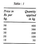
The law of supply is explained with the help of a schedule and a curve. A supply schedule is a statement of the various quantities of a given commodity offered for sale at various prices per unit of time. Table 1 shows a hypothetical supply schedule for apples.
If we depict this supply schedule on a diagram, we have a supply curve S as in Figure 1. The supply curve has a positive slope. It moves upward to the right. The curve S1 shows an increased supply OQ at OP price. It is a curve to the right of and below the original curve S where more is sold at all prices.
The curve S, portrays a decreased supply OQ2 at OP price. It is a curve to the left of and above the original curve S and shows less supply at all prices.

Exceptions:
There are, however, certain exceptions to the law of supply.
ADVERTISEMENTS:
(1) When prices are expected to fall much, sellers will sell more in order to clear their stocks. This is so in the short-run.
(2) Over the long-run, the supply is influenced by changes in costs which are, in turn, affected by changes in technology.
(3) Changes in habits, tastes, fashions, weather, and national and international disturbances also affect the supplies of commodities.
(4) A rise in the price of a good or service sometimes leads to a fall in its supply. This happens particularly in the case of labour-service. When wages rise to a level where the workers feel satisfied, they will work less than before in order to have more leisure. They will also have a tendency to educate their children rather than send them to work.
ADVERTISEMENTS:
The supply curve in such a situation is backward sloping SS1 curve, as illustrated in Figure 2. At WN wage rate, the supply of labour is ON. But when wages start rising, the supply of labour is reduced. At W1M wage rate, the supply of labour is reduced to OM.

Essay # 3. The Elasticity of Supply:
The concept of elasticity is also applicable to supply. The elasticity of supply is the degree of responsiveness of a change in supply to a change in price on the part of sellers. The coefficient of elasticity of supply is
Change in amount supplied/amount supplied ÷ Change in price/Price
∆q/q ÷ ∆p/p = ∆q/∆p × p/q
Where q refers to the amount supplied and p to the price and д represents a change. The coefficient of elasticity of supply is always positive.
ADVERTISEMENTS:
The elasticity of supply can be shown to have five cases:
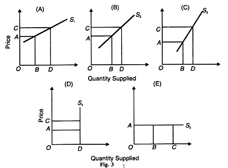
(i) Supply is relatively elastic when a given change in price CA causes a more than proportionate change in the amount supplied BD. S, is a relatively elastic supply curve in Figure 3 (A).
(ii) Elasticity of supply is unity when the change in the amount supplied is in exact proportion to the change in price CA = BD. The curve S2 which is a 45° line represents unit elasticity in Figure 3(B).
(iii) When a given change in price leads to a less than proportionate change in the amount supplied, BD < CA. Supply is relatively inelastic. The curve S3 represents this case in Figure 3 (C).
(iv) Supply is perfectly inelastic when a change in price causes no change in supply whatsoever. The vertical curve S4 shows inelastic supply in Figure 3. (D).
(v) When an infinitely small change in price leads to an infinitely large change in the quantity supplied, supply is perfectly elastic. The horizontal curve S5 in Figure 3 (E) shows perfectly elastic supply.
It’s Measurement:
The elasticity of supply is measured by the point method as in Figure 4.
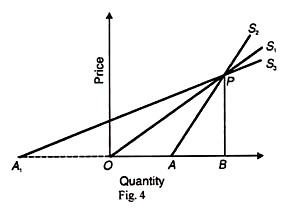
The elasticity of supply at point P on the supply curve S can be measured with the help of the formula:
Es= ∆q/∆p × p/q, Where ∆q/∆p is the slope of the supply
Curve S1 which is OB/ BP and p/q = BP/OB. Thus the elasticity of supply curve S1 at point P is OB/BP × BP/OB= 1 (Unity).
ADVERTISEMENTS:
Similarly, the elasticity of supply at point P on the supply curve S2 is AB/BP × BP/OB= A1B/OB<1 (less than unity).
Also, the elasticity of supply at point P on the supply curve S3 is A1B/BP × BP/Ob = A1B/OB > 1 (greater than unity).
Let us measure the elasticity of supply numerically from Table 1. Suppose the price of commodity Arises from Rs.30 to Rs.50 and its quantity supplied increases from 200 kgs. to 400 kgs. The elasticity of supply is
ES = ∆q/∆p × p/q = 400-200/50-30 × 30/200 = 200/20 × 30/200 = 3/2 or > 1
Now suppose the price of commodity X falls from Rs.50 to Rs.30 and the quantity supplied decreases from 400 kgs to 200 kgs. The elasticity of supply is
ES = ∆q/∆p × p/q = 200-400/30-50 × 50/400 = -200/-20 × 50/400 = 5/4 or > 1
ADVERTISEMENTS:
The price elasticity of supply midway between Rs.50 and Rs.30 in Table 1 can be calculated with the formula of elasticity.
Factors Influencing Supply Elasticity:
Some of the important factors which influence the supply elasticity of a commodity are discussed below:
1. Nature of the Commodity:
If a commodity is perishable, its supply is inelastic. This is because its supply cannot be raised or cut by a rise or fall in its price. On the other hand, the supply of a durable commodity is elastic because its supply can be changed with the change in its price.
2. Cost of production:
If the per unit cost of production increases at a faster rate than the rise in price, the supply will he inelastic. On the other hand, if the per unit cost of production of a commodity increases very slowly in response to a price rise, the supply will be elastic.
3. Time Element:
The longer the time period, the more elastic will be the supply of a commodity. The shorter the time period, the more inelastic will be the supply of the commodity. The supply of a commodity can be increased or decreased in the long run than in the short run.
4. Producers’ Expectations:
If producers expect a rise in the price of a commodity in the future, they will cut down the present supply. As a result, the supply will be inelastic. On the other hand, if they expect the price to fall in the future, they will increase the present supply. Consequently, the supply will become elastic.
Essay # 4. The Short-Run Supply Curve of the Firm and Industry:
The short-run is such a period in which the fixed factors like plants, machinery, etc. cannot be changed. The firm can, therefore, raise output by increasing the quantities of variable factors like labour, raw materials, etc.
The supply curve of a firm shows the various quantities of a commodity offered for sale at various alternative prices. A perfectly competitive firm will sell that output at which its marginal cost equals price (AR = P = MC). Under perfect competition, the price is fixed by the industry for the firm.
Therefore, the price line is parallel to the X- axis as shown by the dotted lines in Figure 5 (A). In the short-run, it must, however, cover its variable cost. Thus the short-run supply curve of the firm is that portion of its marginal cost curve which lies above its average variable cost curve. This is shown in Figure 4 (A) where the SMC curve intersects the AVC curve at point В and OQ2 quantity is sold.
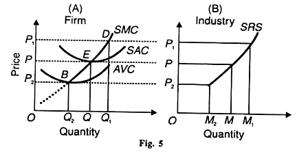
The SMC curve lies below the A VC curve at the volume of output less than this. The firm would not produce below OQ2 since it would not he covering its AVC to the left of point B. At the CP price, the firm will be selling OQ quantity and earning normal profits. At a higher price OP1 it would be earning super normal profits by selling OQ1 units.
Thus that portion of the SMC curve which is rising and lies to the right and above the point of intersection with the AVC curve is the firm’s short-run supply curve. The short-run supply curve of a perfectly competitive industry is the lateral summation of the marginal cost curves of the firms that lie above the minimum points of the AVC curves.
Assuming that the firms in the industry have identical cost curves and there are 1000 firms in it, as shown in Figure 5 (B), the industry’s supply OM, would be OQ2 x 1000 units at the OP2 price, supply OM = OQ x 1000 units at the OP price and supply OM1 = OQ1 x 1000 units at the price OP1 The industry would, however, stop all supplies if the price falls below OP2.
We may conclude that the short-run supply curve of the perfectly competitive industry SRS slopes upward since the short-run marginal cost curves of the firms are positively inclined. In other words, the short- run industry supply curves cannot be downward sloping unless the marginal cost curves of some of the firms are negatively inclined. Such a situation is, however, not possible because the necessary condition for a firm’s equilibrium is that the SMC curve must cut the MR curve from below.
Essay # 5. The Long-Run Supply Curve of the Firm and Industry:
The long-run supply curve of a perfectly competitive industry indicates the various quantities of a product offered at various prices. In the long-run, the firms can change the existing plant and equipment and they can enter or leave the industry, so that price is always equal to both the marginal cost as well as the minimum average cost (Price = LMC = LAC).
However, the entry or exit of firms affects the cost of productive resources and thereby causes shifts in the cost curves of the individual firms. Thus the long-run supply curves can be upward sloping, horizontal or downward sloping, depending upon the law of returns under which the industry is operating.
Increasing-Cost Industry:
An industry is an increasing-cost industry whose long-run supply curve slopes upward from left to right when factor prices rise as industry output expands. Let us suppose that the industry is operating under the law of increasing costs or diminishing returns.
The expansion of the industry by the entry of new firms causes t demand for factors to rise thus increasing their price which, in turn, shifts the cost curves of the firms upward. It means that the minimum point on the average cost curve will be at a higher level than before.
The upward shifting of the cost curves is due to the presence of external diseconomies like rise in the prices of raw materials plant and equipment, wages of labour, etc. This makes the long-run supply curve of the industry slope upward to the right. This is illustrated in Figure 6 (A) and (B) where Panel (A) shows the equilibrium of the firm and Panel (B) equilibrium of the industry.
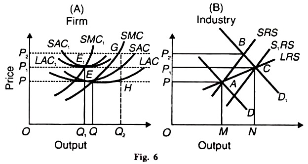
In Panel (A), the initial equilibrium price is OP where each firm produces OQ output at the OP price determined by the industry. Panel (B) shows the determination of OP price in the industry when the short-run supply curve SRS intersects the demand curve D at point A and the entire industry produces OM output which is OQ multiplied by the number of firms. When the demand D to D1 in panel (B) of the figure В, becomes the equilibrium point of the industry. Price goes up to OP2 .The existing firms expand output in the short-run to OQ, when the SMC curve cuts the price line P2 at point G in Panel (A).
The firms earn GH profits per unit. Attracted by these profits new firms enter the industry in the long-run. Since it is an increasing- cost industry, factor prices rise and the cost curves of firms shift up from LAC, SAC and SMC to LAC1, SAC1, and SMC1.
With the expansion of output of the industry the short-run industry supply curve shifts from SRS to SRS1 and cuts the demand curve D1 at point С so that the new equilibrium price is OP1 in Panel (B) at this price OP1 the firm is in equilibrium at point E, where P1 = LAC1 = SMC1 SMC Each firm is producing OQ1 output and the industry output in ON. The initial and new equilibrium points of the industry A and С trace out the long run supply curve LRS which slopes upward to the right indicating that costs rise as the Industry expands, as in Panel (B).
In Figure 6 (A), the higher cost curves LAC1, SAC 1and SMC1 have been shown to shift to the left on the presumption that unmindful of the higher costs of production, the firms produce more because the prices of fixed factors raise less in proportion to the variable factors.
The cost curves will be pushed upward to the rig if the prices of fixed factors rise more than proportionately in the variable factors. The firms will shrink in size and produce less than before. If factor prices rise proportionately, the cost curves will be pushed up straight and the new output of the firms will be the same as before.
Constant-Cost Industry:
An industry is said to be a constant-cost industry if its long-run supply curve is horizontal when factor prices remain constant as industry output expands. A constant-cost industry is subject to both external economies and diseconomies in such a way that they counterbalance each other so that there are constant costs in the lone run. In other words, in such a situation, the supply of various factors is perfectly elastic.
When new firms enter the industry in the long-run, they are able to obtain them at the same prices. Contrariwise, reduction in the number of firms will have no effect on factor prices. Thus, there is no change or shifting of the cost curves.
Under these circumstances, the minimum point on the LAC curve remains unchanged. In Panel (B) of fig-7 the industry is in equilibrium at point A where its short- run supply curve SRS intersects its demand curve D. It produces and sells OM output at OP price.
At this price, the firm is in long run equilibrium at point E where P = LAC = SAC = SMC and is producing OQ output in Panel (A). Suppose the industry demand increases from D to D1 .As a result, the new equilibrium point В sets a higher price OP1.

At this higher price, the existing firms expand output to OQ1 when the SMC curve cuts the price line P1 at point G so that the firms earn GH profit per unit of output. Output Attracted by these profits, new firms will enter the industry; increase the supply and the short-run supply curve of industry shifts from SRS to SRS1 to the right. This establishes the new equilibrium point С with the demand curve D, and the price falls back to OP. At this price, each firm returns to the original long-run equilibrium point E in Panel (A).
This is because under a constant-cost industry, factor prices remain constant and factors are in perfectly elastic supply. By joining the equilibrium points A and C, we trace out the LRS curve in Panel (B) which is horizontal, indicating that costs remain the same as the industry expands.
The expansion of the industry is shown by the increase in output in the long run along the LRS curve from OM to ON, even though the output of each firm is shown to remain constant at OQ. This is due to the increase in the number of firms each producing the same output OQ.
Decreasing-Cost Industry:
In the case of a decreasing-cost industry, the long-run supply curve is downward sloping because factor prices fall as industry output expands. This is illustrated in Figure 8. In Panel (B), the industry is in initial equilibrium at point A with the intersection of D and SRS curves so that OP price is determined ‘ and the industry output is OM.

Industry At this price, each firm is in long-run equilibrium at point E and produces OQ output in Panel (A). With the increase in demand from D to D1, the new equilibrium is at point В and the price rises to OP2. As a result, the existing firms expand output to OQ2 and earn GH profits per unit. Attracted by these profits, new firms enter the industry, expand the industry output and reduce the factor prices so that the industry supply curve shifts from SRS to SRS1.
This establishes the new equilibrium at point С with D1 the curve. By joining points A and C, we trace the downward sloping LRS curve. The price falls to OP which is the result of reduction in factor prices on account of the presence of external economies, such as cheap trained labour, cheap and better marketing and transport facilities, etc.
The presence of external economies leads to reduction in costs so that the cost curves shift downward from LAC, SAC and SMC to LAC1 SAC1 and SMC1 at a lower price OP1 in Panel (B). The firm is in equilibrium at E1 where P1 = LAC1 = SAC1 = SMC1.
The cost curves of each firm have been shown to shift to the right so that its output increases to OQ and the industry output has increased to ON. This means that there has been a reduction in the number of firms resulting from a fall in costs because some firms unable to cover their average costs have been competed away, but others have expanded their outputs.
Essay # 6. Supply Curve under Monopoly or Imperfect Competition:
There is no unique supply curve under imperfect competition or monopoly. The reason is that price is simultaneously determined along with output. Unlike perfect competition, the price is not given to the producer under monopoly.
He is a price-maker who can set the price to his maximum advantage and his output or supply is determined by the consumer demand for his product. It is, therefore, impossible to talk of a supply curve under monopoly. This can be proved with the help of Figures 9 and 10.

Figure 9 shows two demand curves AR1 and AR2 faced by the producer under monopoly. Given his MC curve, the optimum output OQ, is determined when MC=MR1; at point E1. The price is OP1 (= Q1A). When the demand is AR2 the optimum output OQ2 is determined by the equality of MC and MR2 at point E2 .
The price is the same OP1; (= Q2B = Q1A). This shows that the output supplied by the producer under monopoly depends upon the demand conditions for his product and no unique supply curve can be drawn for him.
Figure 10 shows the case where a given output is associated with two different prices. When the demand curve is AR1 OQ output is determined at OP (=QA) price with equilibrium at point E where MC = MR2. When the demand curve is AR2 the same output OQ is determined at point E where MC = MR, but it is sold at a higher price OP1 (=QB).
This is the case when demand differs per period and the same quantity is sold by the producer at different prices. In period I, the demand curve AR1; is elastic and the monopolist sells OQ quantity at OP price. In period 2, the demand curve AR} is less elastic and he sells the same quantity OQ at a higher price OP1.
These two cases show that there is no unique supply curve under monopoly.