
List of top eight examples to illustrate the theory of cost.
Example 1.
The short-run cost function of a company is given by C = 190 + 53 Q, where C is the total cost and Q is the quantity of output.
(i) What is the company’s fixed cost?
(ii) If the company produces 100 units, what is the average variable cost?
ADVERTISEMENTS:
(iii) What is its marginal cost?
(iv) What is its average fixed cost function?
Solution:
The company’s cost function is:
ADVERTISEMENTS:
C = 190 + 53Q …(1)
(i) Since fixed cost is that part of cost of production which is independent of Q, it is evident from (1) that the company’s fixed cost is 190 (units of money).
(ii) Since the company’s variable cost is that part of its total cost which is a function of Q, here the total variable cost (TVC) is
TVC = 53Q …(2)
ADVERTISEMENTS:
Therefore, if Q = 100, TVC = 5,300
And so we have AVC = TVC/Q = 5,300/100 = 53 (units of money)
Actually, since AVC = TVC/Q = 53Q/Q = 53 = constraint, the company’s AVC is 53 (units of money) whatever may be its Q
(iii) Since, by definition, marginal cost is MC = dC/dQ, we obtain from (1): MC = 53 (units of money) = constant.
(iv) By definition, the average fixed cost function (AFC) is: AFC = TFC/Q
Therefore, here, the AFC function is: AFC = 190/Q …(3)
Example 2.
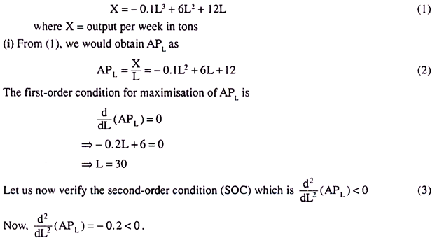
The short-run production function of a firm is X = – 0.1L3 + 6L2 + 12L where X = output per week and L = number of persons employed. Find the values of (i) L that would maximise AP(, (ii) L that would maximise MPL, (iii) quantity of output at minimum AVC and (iv) quantity of output at maximum profit.
Solution:
The short-run production function of the firm is:
ADVERTISEMENTS:
ADVERTISEMENTS:
So the SOC is satisfied.
ADVERTISEMENTS:
Hence the number of persons the firm should employ in order to maximize APL is 30

ADVERTISEMENTS:
ADVERTISEMENTS:
ADVERTISEMENTS:

Therefore, the profit-maximising output is 3,680 tons per week.
Example 3.
Derive the short-run cost function of a firm whose production function is given as:
X = AL1/4K3/4, given PL = 1 and PK = 2, and K is the fixed input and L the variable input in the short-run, If PL increases, ceteris paribus from 1 to 2, then how would the slope of cost function change?
Solution:
The production function of the firm is given as:
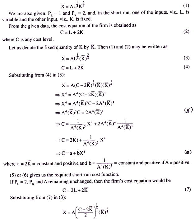

(8) or (9) is the short-run cost function of the firm if PL rises to 2, ceteris paribus. If we compare (5) or (6) and (8) or (9), we come to the conclusion that if PL rises from 1 to 2, ceteris paribus, then the short-run cost function (8) would start from the same point on the vertical axis as the short-run cost function (5), the vertical intercepts of both (5) and (8) being equal to a = 2 K̅. However, if PL rises, the cost function would become steeper than what it was before. For, in the case of (6), we have

To be more precise, in the given example, as P is doubled, ceteris paribus, the slope of the cost function becomes twice as much at each X as that of the initial function.
Example 4.
If x = A![]() is the production function of a firm—
is the production function of a firm—
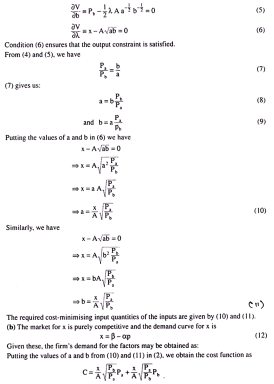
(a) Find the amount of the factors used at given prices Pa and Pb to produce an output x at the smallest cost, (b) In the case of pure competition in the market for x with the demand curve x = β – αp, show that the demands for the factors are

Solution:
(a) The production function of the firm is:

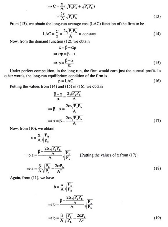
Therefore, the demands for the factors are given by the values of a and b in (18) and (19) respectively. Hence Proved.
Example 5.
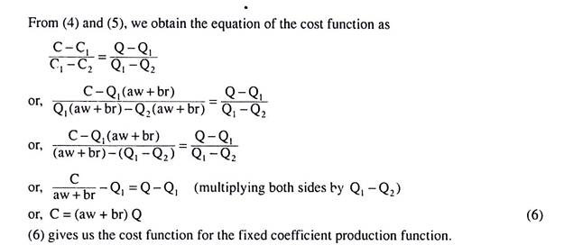
Derive the cost function from the fixed coefficient production function.
Solution.
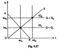
Let us suppose that the fixed coefficient production function is given as:

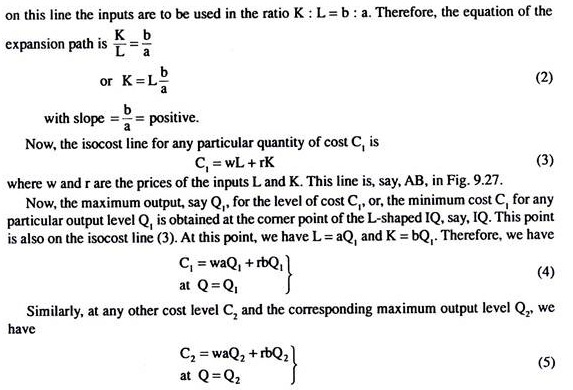
where the inputs are used in a fixed ratio L : K = a : b
For the production function (1), the isoquants (IQs) are L-shaped and the expansion path is a straight line from the origin sloping upward towards right, like OE in Fig. 9.27. At any point
Example 6.
Derive the cost function from the Cobb-Douglas production function.
Solution:
The Cobb-Douglas production function is given by Q = ALαK1 – α (1)
where A and a are constants and the other symbols have their usual meanings.
The cost equation of the firm is:
C = wL + rK (2)
where w and r are the prices of the inputs.
If Q in (1) is any particular quantity of output, then the first-order condition for minimisation of C in (2) subject to the output constraint as given by (1) is

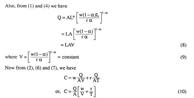
(10) gives us the required cost function for the C-D function (1). The values of the constant V and T in (10) are given in (9) and (7).
Example 7.
If the production functions are:
(a) f(K, L) = min (K, L);
(b) f(K, L) = K + L then find the cost functions.
Solution:
(a) f(K, L) = Min (K, L) is a fixed coefficient production function.
Here we have L : K = 1 : 1, or, L = K, and, therefore, Q = L and Q = K.
Now the cost equation of the firm is
C = wL + rK (where w and r are the prices of the inputs)
or, C = wQ + rQ
or, C = (w + r)Q, which is the required (total) cost function.
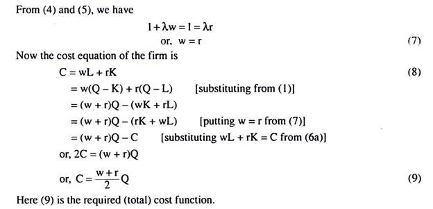
(b) The production function is
Q = K + L (1)
and the isocost equation is
C°= wL + rK (2)
The relevant Lagrange function for maximum output subject to the cost constraint is
V = K + L + λ(wL + rK-C°) (3)
The first order condition for maximum output subject to a given cost, which is same as the minimum cost subject to a given output, is

Example 8.
There are 10 firms in a competitive market. Each firm has a cost function C = 16 + q2. The market demand function is q = 24 – p. Determine the equilibrium price and quantity per firm.
Solution.
The cost function of each firm is:
C = 16 + q2 (1)
Therefore, the firm’s marginal cost (MC) function is
MC = dC/dq = 2q.
Therefore, the short-run supply (SRS) curve of the industry, which is the horizontal summation of the short-run MC curves of 10 firms is

Therefore, from (3a), p = 24 – 20 = 4 (Rs).
Also, the output of each firm = 20/10 = 2 units.
Therefore, the equilibrium price and output per firm are Rs 4 and 2 units, respectively.