Examples of Monopoly | Microeconomics

List of top five examples of monopoly.

Example 1.

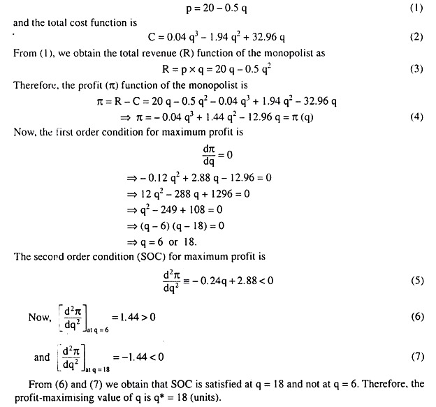
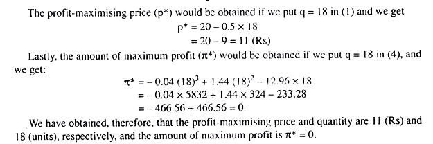
Determine the maximum profit and the corresponding price and quantity for a monopolist whose demand and cost functions are p = 20 – 0.5q and C = 0.04q³ -1,94q² + 32.96q, respectively.

Solution.

The demand or average revenue (AR) function of the monopolist is

Example 2.

Let the demand and cost functions of a multi-plant monopolist be p = a – b (q₁ + q₂), C₁ = α₁q₁ + β₁q₁² and C₂ = a₂q₂ + β₂q₂² where all the parameters are positive. Assume that an autonomous increase in demand increases the value of a, leaving the other parameters un­changed. Show that output will increase in both plants with a greater increase in the plant in which the marginal cost is increasing less faster.

Solution.

The demand or the average revenue (AR) function of the monopolist is

And the total cost functions in the two plants are

From (1) we have

R (total revenue) = p (q₁ +q₂) = a (q₁ + q₂) – b (q₁ + q₂)²                          (4)

Now, the profit function of the monopolist is

From (5), we may derive the FOCs for maximum profit as

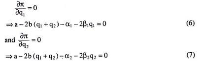
Next, taking total differential of (6) and (7) with respect of q₁, q₂ and a, we obtain

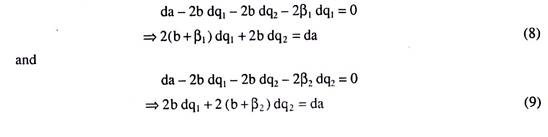
Now, solving (8) and (9) by Cramer’s rule, we obtain

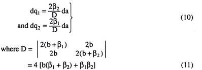
Here, since all the parameters are given to be positive, we have D > 0, and therefore, from (10) we obtain

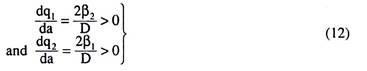
Eqn. (12) gives us that a s ‘a’ increases on account of an assumed autonomous increase in demand, both q₁ and q₂ get increased, which is what we have to prove here.

Also, (12) gives us, if the slope, 2β₁, of the MC₁ function of plant 1 is smaller than the slope, 2β₂, of the MC₂ function of plant 2, then dq₁/da would be larger than dq₂/da, i.e., an increase in ‘a’ would result in a large increase in output in the plant (here plant 1) in which MC is increasing less fast.

Let us note that the MC function of plant 1 is MC₁ = dC₁/dq₁ = α1 + 2β₁q₁, and the MC function of Plant 2 is MC2 = dC₂/dq₂ = α2 + 2β₂q₂. It is obvious that the slopes of the MC₁ and MC₂ functions are 2β₁ and 2β₂, respectively.

Example 3.

A monopolist sells his output in two distinct markets between which price discrimi­nation is possible.

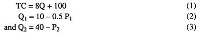
His total cost curve and the two demand curves are given by:

TC = 8Q + 100 ; Q₁ = 10 – 0.5 P₁ ; Q₂ = 40 – P₂

(i) Calculate the profit-maximising values of P₁, P₂, Q₁ and Q₂.

(ii) Verify that higher price is charged in the market with lower price-elasticity of demand.

Solution.

The total cost curve and the two demand curves of the monopolist are

From (2) and (3) we obtain (4) and (5) below:

From (4) and (5), we obtain the total revenue and marginal revenue functions, TR₁ and MR₁, for market 1, and those functions, TR₂ and MR₂, for market 2 as derived below:

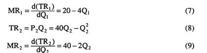
Also, from (1), we obtain the MC function of the monopolist is

Now, the FOC for maximum profit of the monopolist is

From (12), we obtain Q₁ = 3 units Q₂ = 16 units. Putting these values in (4) and (5), we obtain: P₁ = 14 (Rs.) and P₂ = 24 (RS.). These are the required profit-maximising value of P₁, P₂, Q₁ and Q₂.

Lastly, the slope of the demand curve (4) and (5) are -2 and -1, respectively. Now, the numerical coefficients (e₁ and e₂) of price-elasticity of demand in markets 1 and 2 are

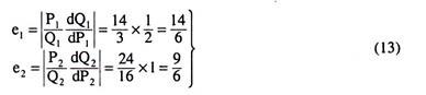
Eqn. (13) gives us, e₁ < e₂, and we already have, P₂ = 24 > P1 = 14. That is, it is verified here that higher price is charged in the market (here market 2) with lower price-elasticity of demand.

Example 4.

Determine the maximum profit and the corresponding marginal price and quantity for a perfectly discriminating monopolist whose demand and cost functions are p = 2,200 – 60q and C = 0.5q³ – 61,5q² + 2740q, respectively.

Solution.

The demand and cost functions of a perfectly discriminating monopolist are, respectively,

P = 2,200 – 60q                                              (1)

and C = 0.5q³ – 61.5q² + 2,740q              (2)

We have to determine the amount of maximum profit and the corresponding marginal price and quantity. We may do this in the following way.

By definition, under perfect price discrimination, the demand curve of the monopolist is identical with his marginal revenue (MR) curve.

Therefore, (1) itself gives us the MR function, and we may write:

MR = 2,200 – 60q                                          (3)

Also, from (2), we have the MC function as

MC = dC/dq = 1.5q² – 123q + 2,740          (4)

Now, the FOC for maximum profit is

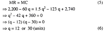
Here we have two values of q. Let us see which of them satisfies the SOC for maximum profit, which is given by

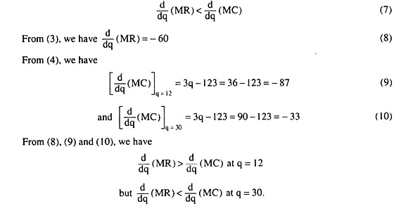
Therefore, of the two values of q, 12 and 30, q = 30 satisfies the SOC for maximum profit and so we may accept this value, i.e., q = 30 (units) as the profit-maximising quantity. Putting this value, q = 30, in (1), we obtain the marginal price, i.e., the price of the 30^th unit to be p = 2,200 – 60 x 30 = 400 (Rs).

Lastly, in order to have the value of maximum profit, we may proceed in the following way:

At q = 30, the TR of the firm is

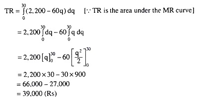
Next, we may obtain TC at q = 30 if we put this value of q in eq. (2), or, if we integrate the MC function for q = 30. If we go by the latter method, we have

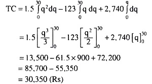
Therefore, the maximum profit (π)

π = TR – TC = 39,000 – 30,350

= 8,650 (Rs)

So, the amount of maximum profit, i.e., the profit at q = 30 is Rs 8,650.

Therefore, we have obtained at the maximum profit point:

Marginal price = 400 (Rs), output quantity

= 30 (units) and the amount of (maximum) profit

= 8,650 (Rs)

Example 5.

Suppose that a revenue maximising monopolist requires a profit of at least 1,500 (Rs). His demand and cost functions are p = 304 – 2q and TC = 500 + 4q + 8q². Determine his output level and price.

Contrast these values with those that would be achieved under profit maximisation.

Solution.

The demand or the average revenue (AR) function of the monopolist is

 

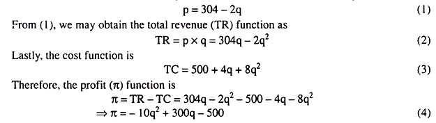
Here, we are given that the goal of the monopolist is to maximise revenue subject to a profit constraint. The constraint on profit here is given to be π ≥ 1,500 (Rs).

In this case, the minimum required profit, πc (= Rs 1,500 here) must lie between the maximum attainable profit, and the profit at the point of maximum revenue, π_rev. Since revenue would increase as π approaches π_max from πc, the revenue-maximising monopolist would stick to π = π_c (= Rs 1,500) although the condition is π ≥ π_c.

In view of above, we may write (4) as:

– 10 q² + 300 q-500= 1,500

⇒ (q-20) (q- 10) = 0

⇒ q = 20 (units) or 10 (units).

Now, when q = 20, TR = 5,280 (Rs)

and when q = 10, TR = 2,840 (Rs)

So the revenue-maximising monopolist would accept the larger TR, i.e., TR = 5,280 (Rs) at q = 20 (units). Putting this value of q in (1), we obtain: p = 304 – 40 = 264 (Rs).

We may now obtain the price-output combination of the monopolist under profit- maximisation. The FOC for maximum profit is

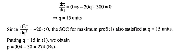
If we now compare the price-output combination (p = 264, q = 20) under revenue maximisation with the combination (p = 274, q = 15) under profit maximisation, we find that the price in the former case is lower by Rs 10 and the quantity higher by 5 units than those in the latter case.