Cost in Short Run and Long Run (With Diagram)

In this article we will discuss about Cost in Short Run and Long Run.

Cost in Short Run:

It may be noted at the outset that, in cost ac­counting, we adopt functional classification of cost. But in economics we adopt a different type of clas­sification, viz., behavioural classification-cost beha­viour is related to output changes.

In the short run the levels of usage of some input are fixed and costs associated with these fixed inputs must be incurred regardless of the level of output produced. Other costs do vary with the level of output produced by the firm during that time period.

The sum-total of all such costs-fixed and variable, explicit and implicit- is short-run total cost. It is also possible to speak of semi-fixed or semi-variable cost such as wages and compensation of foremen and electricity bill. For the sake of simplicity we assume that all short run costs to fall into one of two categories, fixed or variable.

Short-Run Total Cost:

A typical short-run total cost curve (STC) is shown in Fig. 14.3. This curve indicates the firm’s total cost of production for each level of output when the usage of one or more of the firm’s resources remains fixed.

When output is zero, cost is positive because fixed cost has to be incurred regardless of output. Examples of such costs are rent of land, deprecia­tion charges, license fee, interest on loan, etc. They are called unavoidable contractual costs. Such costs remain contractually fixed and so cannot be avoided in the short run.

The only way to avoid such costs is

by going into liquidation. The total fixed cost (TFC) curve is a horizontal straight line. Total variable is the difference between total cost and fixed cost. The total variable cost curve (TVC) starts from the origin, because such cost varies with the level of output and hence are avoidable. Examples are electricity tariff, wages and compensation of casual workers, cost of raw materials etc.

In Fig. 14.3 the total cost (OC) of producing Q units of output is total fixed cost OF plus total vari­able cost (FC).

Clearly, variable cost and, therefore, total cost must increase with an increase in output. We also see that variable cost first increase at a decreasing rate (the slope of STC decreases) then increase at an increasing rate (the slope of STC increases). This cost structure is accounted for by the law of Variable Proportions.

Average and Marginal Cost:

One can gain a better insight into the firm’s cost structure by analysing the behaviour of short-run average and marginal costs. We may first consider average fixed cost (AFC).

Average fixed cost is total fixed cost divided by output,

i.e., AFC = TFC /Q

Since total fixed cost does not vary with output average fixed cost is a constant amount divided by output. Average fixed cost is relatively high at very low output levels. However, with gradual increase in output, AFC continues to fall as output increases, approaching zero as output becomes very large. In Fig. 14.4, we observe that the AFC curve takes the shape of a rectangular hyperbola.

We now consider average variable cost (AVC) which is arrived at by dividing total variable cost by output,

i.e., AVC= — TVC/Q

In Fig. 14.4, AVC is a typical average variable cost curve. Average variable cost first falls, reaches a minimum point (at output level Q₂) and subse­quently increases.

The next important concept is one of average total cost (ATC).

It is calculated by dividing total cost by output,

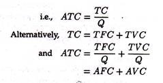
It is, therefore, the sum of average fixed cost and average variable cost.

The ATC curve, illustrated, is U-shaped in Fig. 14.4 because the AVC cost curve is U-shaped. This is accounted for by the Law of Variable Propor­tions. It first declines, reaches a minimum (at Q₃ units of output) and subsequently rises. The min­imum point on ATC is reached at a larger output than at which AVC attains its minimum. This point can easily be proved.

ATC = AFC + AVC

We know that and that average fixed cost continuously falls over the whole range of output. Thus, ATC declines at first because both AFC and AVC are falling. Even when AVC begins to rise after Q₂, the decrease in AFC continues to drive down ATC as output in­creases. However, an output of Q₃ is finally reached, at which the increase in AVC overcomes the decrease in AFC, and ATC starts rising.

Since ATC = AFC + AVC, the vertical distance be­tween average total cost and average variable cost measures average fixed cost. Since AFC declines over the entire range of output. AVC becomes closer and closer to ATC as output increases.

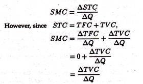
We may finally consider short-run marginal cost (SMC). Marginal cost is the change in short-run total cost attributable to an extra unit of output: or

Short-run marginal cost refers to the change in cost that results from a change in output when the usage of the variable factor changes. As Fig. 14.4 shows, marginal cost first declines, reaches a min­imum at Q_x (note that minimum marginal cost is attained at a level of output less than that at which AVC and ATC attain their minimum) and rises there­after.

The marginal cost curve intersects AVC and ATC at their respective minimum points. This result fol­lows from the definitions of the cost curves. If mar­ginal cost curve lies below average variable cost cur­ve the implication is clear: each additional unit of output adds less to total cost than the average vari­able cost.

Thus average variable cost has to fall. So long as MC is above AVC, each additional unit of output adds more to total cost than AVC. Thus, in this case, AVC must rise.

Thus when MC is less than AVC, average vari­able cost is falling. When MC is greater than AVC, average variable cost is rising. Thus MC must equal AVC at the minimum point of AVC. Exactly the same reasoning would apply to show MC crosses ATC at the minimum point of the latter curve.

a. Short-run Cost Functions:

Summary of the Main Points All the important short-run cost relations may now be summed up:

The total cost function may be expressed as:

TC = k + ƒ(Q) where k is total fixed cost which is a constant, and ƒ(Q) is total variable cost which is a function of output.

ATC = k/Q + ƒ(Q)/ Q = AFC + AVC. Since k is a constant and Q gradually increases, the ratio k/Q falls. Hence the AFC curve is a rectangular hyperbola.

Here

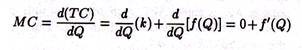
where ƒ'(Q) is the change in TVC and may be called marginal variable cost (MVC). Thus, it is clear that MC refers to MVC and has no relation to fixed cost. Since business decisions are largely governed by marginal cost, and marginal costs have no relation to fixed cost, it logically follows costs do not affect business decisions.

b. Relation between MC and AC:

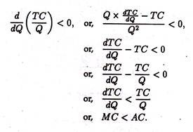
There is a close relation between MC and AC. When AC is falling, MC is less than AC. This can be proved as follows:

When AC is falling,

c. Cost Elasticity:

On the basis of the relation between MC and AC we can develop a new concept, viz., the concept of cost elasticity. It measures the responsiveness of total cost to a small change in the level of output.

It can be expressed as:

So it is the ratio of MC to AC.

The properties of the average and marginal cost curves and their relationship to each other are as de­scribed in Fig. 14.4. From the diagram the following relationships can be discovered.

(1) AFC declines continuously, approaching both axes asymptomatically (as shown by the de­creasing distance between ATC and AVC) and is a rectangular hyperbola.

(2) AVC first declines, reach­es a minimum at Q₂and rises thereafter. When AVC is at its minimum, MC equals AVC.

(3) ATC first declines, reaches a minimum at Q₃, and rises there­after. When ATC is at its minimum, MC equals ATC.

(4) MC first declines, reaches a minimum at Q₁, and rises thereafter. MC equals both AVC and ATC when these curves are at their minimum values.

The low­est point of the AVC curve is called the shut (close)- down point and that of the ATC curve the break-even point. These two concepts will be discussed in the context of market structure and pricing. Finally, we see that MC lies below both AVC and ATC over the range in which these curves decline; contrarily, MC lies above them when they are rising.

Table 14.2 numerically illustrates the character­istics of all the cost curves. Column (5) shows that average fixed cost decreases over the entire range of output. Columns (6) and (7) depict that both av­erage variable and average total cost first decrease, then increase, with average variable cost attaining a minimum at a lower output than that at which av­erage total cost reaches its minimum. Column (8) shows that marginal cost per 100 units is the incre­mental increase in total cost and variable cost.

If we compare columns (6) and (8) we see that marginal cost (per unit) is below average variable and aver­age total cost when each is falling and is greater than each when AVC and ATC are rising.

Long-Run Costs: The Planning Horizon:

We may recall from our discussion of produc­tion theory that the long run does not refer to ‘some date in the future. Instead, the long run simply refers to a period of time during which all inputs can be varied.

Therefore, a decision has to be made by the owner and/or manager of the firm about the scale of operation, that is, the size of the firm. In order to be able to make this decision the manager must have knowledge about the cost of producing each relevant level of output. We shall now discover how to determine these long-run costs.’

Derivation of Cost Schedules from a Production Function:

For the sake of analysis, we may assume that the firm’s level of usage of the inputs does not affect the input (factor) prices. We also assume that the firm’s manager has already evaluated the production func­tion for each level of output in the feasible range and has derived an expansion path.

For the sake of analytical simplicity, we may assume that the firm uses only two variable factors, labour and capital, that cost Rs. 5 and Rs. 10 per unit, respectively.

The characteristics of a derived expansion path are shown in Columns 1, 2 and 3 of Table 14.4. In column (1) we see seven output levels and in Columns (2) and (3) we see the optimal combinations of labour and capital respectively for each level of output, at the existing factor prices.

These combinations enable us to locate seven points on the expansion path.

Column (4) shows the total cost of producing each level of output at the lowest possible cost. For example, for producing 300 units of output, the least cost combination of inputs is 20 units of labour and 10 of capital. At existing factor prices, the total cost is Rs. 200. Here, Column (4) is a least-cost schedule for various levels of production.

In Column (5), we show average cost which is obtained by dividing total cost figures of Column (4) by the corresponding output figures of Column (1). Thus, when output is 100, average cost is Rs. 120/100 = Rs. 1.20. All other figures of Column (5) are derived in a similar way.

From column (5) we derive an important characteristic of long-run average cost: average cost first declines, reaches a minimum, then rises, as in the short-run. In Column (6) we show long-run marginal cost figures.

Each such figure is arrived at by dividing change in total cost by change in output. For example, when output increases from Rs. 100 to Rs. 200, the total cost increases from Rs. 120 to Rs. 140. Therefore, marginal cost (per unit) is Rs. 20/100 = Re. 0.20. Similarly, when output increases from 600 to 700 units, MC per unit is 720-560/100 =160/100 =1.60

Column (6) depicts the behaviour of per unit MC: marginal cost first decreases then increases, as in the short run.

We may now show the relationship between the expansion path and long-run cost graphically. In Fig. 14.6 two inputs, K and L, are measured along the two axes. The fixed factor price ratio is represented by the slope of the isocost lines I₁I’₁, l₂l’₂ and so on. Finally, the known production function gives us the isoquant map, represented by Q₁, Q₂ and so forth.

From our earlier discussion of long-run produc­tion function we know that, when all inputs are vari­able (that is, in long-run), the manager will choose the least cost combinations of producing each level of output. In Fig. 14.6, we see that the locus of all such combinations is expansion path OP’ B’R’S’.

Given the factor-price ratio and the production func­tion (which is determined by the state of technol­ogy), the expansion path shows the combinations of inputs that enables the firm to produce each level of output at the lowest cost.

We may now relate this expansion path to a long-run total cost (LRTC) curve. Fig. 14.7 shows the ‘least cost curve’ associated with expansion path in Fig. 14.6. This least cost curve is the long-run to­tal cost curve. Points P,B,R and S are associated with points P’, B’, R’ and S’ on the expansion path. For example, in Fig. 14.6 the least cost combination of in­puts that can produce Q₁ is K₁ units of capital and L₁ units of labour.

Thus, in Fig. 14.7, minimum pos­sible cost of producing Q₁ units of output is TC₁, which is K₁ + wL₁, i.e., the price of capital (or the rate of interest) times K₁, plus the price of labour (or the wage rate) times L₁. Every other point on LRTC is derived in a similar way.

Since the long run permits capital-labour substi­tution, the firm may choose different combinations of these two inputs to produce different levels of output. Thus, totally different production processes may be used to produce (say) Q ₁ and Q₂ units of output at the lowest attainable cost.

On the basis of this diagram we may suggest a definition of the long run total cost. The time period during which even/thing (except factor prices and the state of technology or art of production) is variable is called the long run and the associated curve that shows the minimum cost of producing each level of output is called the long- run total cost curve.

The shape of the long-run total cost (LRTC) cur­ve depends on two factors: the production func­tion and the existing factor prices. Table 14.4 and Fig. 14.7 reflect two of the commonly assumed char­acteristics of long-run total costs. First, costs and output are directly related; that is, the LRTC curve has a positive slope. But, since there is no fixed cost in the long run, the long run total cost curve starts from the origin.

Another characteristic of LRTC is that costs first increase at a decreasing rate (until point B in Fig. 14.7), and an increasing rate thereafter. Since the slope of the total cost curve measures marginal cost, the implication is that long-run marginal cost first decreases and then increases. It may be added that all implicit costs of production are included in the LRTC curve.

Long-Run Average and Marginal Costs:

We turn now to distinguish between long run average and marginal costs.

Long-run average cost is arrived at by dividing the total cost of producing a particular output by the number of units produced:

LRTC= LRTC/Q

Long-run marginal cost is the extra total cost of producing an additional unit of output when all inputs are optimally adjusted:

LRTC= ∆ LRTC /∆Q

It, therefore, measures the change in total cost per unit of output as the firm moves along the long run total cost curve (or the expansion path).

Fig. 14.8 illustrates typical long-run average and marginal cost curves. They have essentially the same shape and relation to each other as in the short run. Long-run average cost first declines, reaches a min­imum (at Q₂ in Fig. 14.8), then increases. Long-run marginal cost first declines, reaches minimum at a lower output than that associated with minimum av­erage cost (Q₁ in Fig. 14.8), and increases thereafter.

The marginal cost intersects the average cost curve at its lowest point (L in Fig. 14.8) as in the short-run. The reason is also the same. The reason has been aptly summarized by Maurice and Smithson thus: “When marginal cost is less than average cost, each additional unit produced adds less than average cost to total cost; so average cost must decrease.

When marginal cost is greater than average cost, each ad­ditional unit of the good produced adds more than average cost to total cost; so average cost must be increasing over this range of output. Thus marginal cost must be equal to average cost when average cost is at its minimum”.

The Shape of the LAC: Economies and Diseconomies of Scale:

The shape of the long-run average cost depends on certain advantages and disadvantages associated with large scale production. These are known as economies and diseconomies of scale.

Economies of Scale:

Various factors may give rise to economies of scale, that is, to decreasing long-run average costs of production.

Greater Specialization of Resources:

With an expansion of a firm’s scale of oper­ation, its opportunities for specialization—whether performed by men or by machines—are greatly en­hanced. It is because a large-scale firm can often divide the tasks and work to be done more readily than a small-scale firm.

More Efficient Utilization of Equipment:

In some industries, the technology of produc­tion is such that a large unit of costly equipment has to be used. The production of automobiles, steel and refined petroleum are obvious examples.

In such in­dustries, companies must be able to afford whatever equipment is necessary and must be able to use it efficiently by spreading the cost per unit over a suf­ficiently large volume of output. A small-scale firm cannot ordinarily do these things.

Reduced Unit Costs of Inputs:

A large-scale firm can often buy its inputs-such as its raw materials-at a cheaper price per unit and thus gets discounts on bulk purchases. Moreover, for certain types of equipment, the price per unit of capacity is often much less than larger sizes pur­chased.

For instance, the construction cost per square foot for a large factory is usually less than that for a small one. Again, the price per horsepower of various electric motors varies inversely with the amount of horsepower.

Utilization of by-products:

In certain industries, larger-scale firms can make effective use of many by-products that would go waste in a small firm. A typical example is the sugar industry, where by-products like molasses and bagasse are made use of.

Growth of Auxiliary Facilities:

In certain places, an expanding firm often ben­efits from, or encourages other firms to develop, an­cillary facilities, such as warehousing, marketing, and transportation systems, thus saving the grow­ing firm considerable costs. For example, commer­cial and industrial establishments often benefit from improved transportation and warehousing facilities.

Diseconomies of Scale:

With continuous expansion of the scale of oper­ation of a firm, a point may ultimately be reached when diseconomies of scale begin to exercise a more than offsetting effect on the firm’s cost curve. As a result, the long-run average cost curve starts to rise.

This is attributable to the following two main rea­sons:

Decision-Making Role of Management:

As a firm becomes larger, heavier burdens are placed on the management so that eventually this resource input is overworked relative to others and ‘diminishing returns’ to management set in. In fact, management is an indivisible input which is not ca­pable of continuous variation. With increase in the size of organisation there occurs delay in decision-making.

Competition for Resources:

Rising long-run average costs can occur as a growing firm increasingly bids labour or other re­sources away from other industries. In the real world, it is very difficult, if not virtu­ally impossible, to determine just when diseconomi­es of scale are encountered and when they become strong enough to outweigh the economies of scale.

In business where economies of scale are negligible, diseconomies may soon assume paramount signifi­cance causing LAC to turn up at a relatively small volume of output. Panel A of Fig. 14.9 shows a long run average cost curve for a firm of this type. In other cases, economies of scale assume strate­gic significance.

Even after the efficiency of man­agement starts declining, technological economies of scale may offset the diseconomies over a wide range of output. Thus, the LAC curve may not slope up­ward until a very large volume of output is pro­duced. This case (typified by the so-called natural monopolies) is illustrated in Panel B of Fig. 14.9.

In many actual situations, however, neither of these extremes describes the behaviour of LAC. A very modest scale of operation may not set in until a very large volume of output is produced. In such a situation, LAC would have a long horizontal sec­tion as shown in Panel C of Fig. 14.9.

It is widely agreed by economists and business executives that this type of LAC curve describes many production processes in the real commercial world. For theoretical analysis, however, we continue to assume a “rep­resentative” LAC, such as that illustrated earlier in Fig. 14.8.

Average Cost in the Long Run: Smooth Envelope Case:

We know that in the short-run the firm has a fixed plant and it has a short run U-shaped cost curve SAC. If a new and larger plant is built, the new SAC will be drawn further to the right.

We as­sume that the firm is still in the planning stage and yet to undertake any fixed commitment. It can now draw all possible different U-shaped SAC curves, from which to choose one SAC for each specified level of output that promises the lowest cost. As out­put increases, the firm moves to a new SAC curve.

In the long run, the firm can change the size of the plant. Starting from zero output level, succes­sively larger plants typically have lower and lower ATC up to some output level and then successively higher ATC curves beyond. The three representative ATC curves associated with the three successively larger plants are shown in Fig. 14.11(a).

Plant I is the best plant for output levels less than 900 units because its AC curve is the lowest to the left of point a. Plant II is the best plant size for output levels between 900 to 2,000 units, because its AC curve is the lowest between point a and b. Plant III is the best plant size for output levels greater than 2,000 units, since its AC curve is the lowest beyond point b.

If these are only three possible plant sizes, the long run ATC curve will consist of the segments of Plant I’s AC curve up to point a, the segment of plant II’s AC curve between points a and b, and the segment of Plant Ill’s AC curve from point of b and so on. The thick LAC is composed of the three lowest branches of SACs. This is why the LAC is called the envelope curve.

Fig. 14.11(b) is the smooth envelope case. Writes Samuelson: “In the long run, a firm can choose its best plant sizes and its lower envelope curve.” Since there is an infinite number of choices, we get LAC as a smooth envelope. And, as in the short-run, we can derive LMC from LAC, and LMC emerges from the minimum point of LAC with a smoother slope than the SMC curve.