Empirical Evidence on the Shape of Costs

There are various types of empirical cost studies: statistical cost studies, studies based on questionnaires to firms, engineering cost studies, studies based on the survivor technique’.

The majority of the empirical cost studies suggest that the U-shaped costs postulated by the traditional theory are not observed in the real world.

Two major results emerge predominantly from most studies. Firstly, the short-run TVC is best approximated with a straight (positively-sloping) line.

This means that the AVC and the MC are constant over a fairly wide range of output. Secondly, in the long run the average costs fall sharply over low levels of output and subsequently remain practically constant as the scale of output increases. This means that the long-run cost is L-shaped rather than U-shaped. Only in very few cases were diseconomies of scale observed, and these at very high levels of output.

Of course, all the sources of evidence can and have been attacked on various grounds, some justified and others unjustified. However, the fact that so many diverse sources of evidence point in general to the same direction (that is, lead to broadly similar con­clusions) regarding the shape of costs in practice, surely suggests that the strictly U-shaped cost curves of traditional theory do not adequately represent reality.

A. Statistical Cost Studies:

Statistical cost studies consist in the application of regression analysis to time series or cross-section data. Time-series data include observations on different magnitudes (output, costs, prices, etc.) of a firm over time. Cross-section data give information on the inputs, costs, outputs and other relevant magnitudes of a group of firms at a given point of time.

In principle one can estimate short-run and long-run cost functions either from time series or from cross-section data. We may estimate a short-run cost-function either from time-series data of a single firm over a period during which the firm has a given plant capacity which it has been utilizing at different levels due, for example, to demand fluctuations; or a cross-section sample of firms of the same plant capacity, each of them operating at a different level of output for any reason (for example, due to consumers’ preferences, market-sharing agreements, etc.). Due to the difficulties in obtaining a cross-section sample of firms fulfilling the above requirements, short-run cost functions are typically estimated from time-series data of a single firm whose plant has remained the same during the period covered by the sample.

We may estimate a long-run Cost function either from a time-series sample including the cost-output data of a single firm whose scale of operations has been expanding (with the same state of technology); or a cross-section sample of firms with different plant sizes, each being operated optimally (at its minimum cost level).

Given that over time technology changes, time-series data are not appropriate for the estimation of long-run cost curves. Thus, for long-run statistical cost estimation, cross-sectional analysis is typically used in an attempt to overcome the problem of changing technology, since presumably ‘the state of arts’ is given at any one point of time.

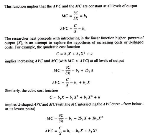
The procedure adopted in statistical cost studies may be outlined as follows. Once the data are collected and appropriately processed (see below) the researcher typically starts by fitting a linear function to the cost-output observations

C = b₁X₁ + u

Where C = total variable cost

X = output (measured in physical volume)

u = a random variable which absorbs (mainly) the influence on costs of all the factors which do not appear explicitly in the cost function.

A comprehensive summary and critique of a wide range of statistical cost studies is given by J. Johnston in his classic work. The evidence from most statistical studies is that in the short run the AVC is constant over a considerable range of output, while in the long run the AC is in general L-shaped. The results of statistical cost studies have been criticized on grounds of their interpreta­tion, data limitations, and omission or inadequate treatment of important explanatory variables (misspecification of the cost function).

Interpretation problems:

The nature of the data:

Statistical cost studies are based on accounting data which differ from the opportunity costs ideally required for the estimation of theoretical cost functions. Accounting data do not include several items which constitute costs in the economist’s view. For example, profit is not included in the accountant’s costs, and the same holds for all imputed costs, which do not involve actual payments.

Thus the statistical cost functions, based on ex post data (realized accounting data), cannot refute the U-shape of costs of the traditional theory, which show the ex ante relationship between cost and output. The statistical results reflect the simple fact that firms in the short run operate within their planned capacity range, and do not go beyond their capacity limits, precisely because they know that beyond these limits costs rise sharply.

Similarly, the evidence of L-shaped long-run costs reflects the actual costs up to levels of outputs so far experienced, and the fact that firms do not expand beyond these levels because they believe that at larger scales of output they will be faced with diseconomies of scale (increasing costs).

The length of the time period:

Ideally the length of the time period should cover the complete production cycle of the commodity. However, the time period of the accoun­tants does not coincide with the true time period over which the production cycle is completed. Usually the accounting data are aggregate data for two or many production periods, and this aggregation may impart some bias towards linearity of the estimated cost functions.

Coverage of cost studies:

Statistical cost studies refer mostly to public companies, which are completely different to companies in the competitive industries. Consequently the evidence cannot be generalized to apply to all industries.

Data deficiencies:

Accounting data are not appropriate for estimating theoretical cost functions not only because they are ex post (realized) expenditures (and not opportunity costs), but for several additional reasons.

Depreciation expenses:

Among the variable costs one should include the user’s cost of the capital equipment. Accounting data give full depreciation figures which include not only the user’s cost but also the obsolescence (or time) costs of the equipment. Further­more, in general accountants use the linear depreciation method, while in the real world depreciation and running expenses of fixed capital are non-linear they increase as the age of the machinery increases.

Allocation of costs:

Costs should be correctly allocated to outputs. However, the allo­cation of semi-fixed costs (which are included in the dependent variable (TVC) of the cost function) are often allocated by accountants to the various products on the basis of some rule of thumb, so that there is not exact correspondence between the output and its reported costs of production.

Cost functions of multiproduct firms:

With multiproduct firms one should estimate a separate cost function for each product. However, the required data either are not available or are not accurate due to the usually ad hoc allocation of joint costs to the various products. Thus researchers tend to estimate an aggregate cost function for all the products of the firm. Such functions are not reliable because of the ‘output index’ which is used as the dependent variable.

The index of output is a weighted index of the various products, the weights being the average cost of the individual products. Under these conditions what one is really measuring is a ‘circular’ relation, some sort of identity rather than a causal relationship, since

C = f(X)

and so that

C = f(AC)

Specification of the cost functions:

The cost curves assume constant technology and constant prices of inputs. If these factors change the cost curves will shift. Statistical cost studies have been criticized for failing to deal adequately with changes in technology and in factor prices.

Changes in technology:

We said that short-run cost curves are typically estimated from time series data of a single firm whose scale of plant has remained constant over the sample period. It is assumed by researchers that the requirement of constant technology is automatically fulfilled from the nature of the time-series data. This, however, may not be true.

A firm may report the same plant size, while the physical units of its equipment have been replaced with more advanced pieces of machinery. For example, a textile firm may have kept its capacity constant while having replaced several obsolete manual weaving machines (which have been fully depreciated) with a single automated machine. This replacement constitutes a change in technology which, if not accounted for, will distort the cost-output relationship.

When using a cross-section sample of firms of different sizes for the estimation of the long-run cost curve, it is assumed that the problem of changing technology is solved, since the available methods of production (‘state of arts’) are known to all firms technology in a cross-section sample is constant in the sense of common knowledge of the ‘state of arts’ at any one time.

This, however, does not mean that all firms in the cross-section sample use equally advanced methods of production. Some firms use modern while others use obsolete methods of production. Under these conditions the problem of differences in technology is brushed away by researchers, by the convenient assumption that technology (i.e. age of plant) is randomly distributed among firms some small firms have obsolete technology while others have advanced technology, and the same is assumed to hold for all firm sizes.

If this assumption is true, differences in the technology of the firms are absorbed by the random variable u and do not affect the cost-output relation. However, this assumption may not be justified in the real world. Indeed it is conceivable that large firms have lower costs because they have more advanced technology. If this is the case, the estimated long-run cost function does not reflect the theoretical cost-output relationship.

In summary, the cost curves, both short-run and long-run, shift continuously due to improvements in technology and the ‘quality’ of the factors of production. These shifts have not been accounted for in estimating the cost curves. Hence the estimated sta­tistical functions are in fact obtained from ‘joining’ points belonging to shifting cost curves, and do not show the theoretical shape of costs.

Changes in factor prices:

Cost functions have been criticized for not dealing adequately with the problem of changes of the prices of factors of production. Time-series data, used in estimating SR cost curves, have in fact been deflated. But the price indexes used were not the ideally required ones, and thus the estimates have a bias. Johnston¹ has argued that the bias involved in the adopted deflating procedures does not necessarily invalidate the statistical findings, since it is not at all clear that the bias should be towards linearity of the cost-output relation.

Cross-section studies are thought to avoid the problem of price changes, since prices are given at any one time. This is true if the firms included in the sample are in the same location. However, cross-section samples include firms in different locations.

If factor prices are different in the various locations they should be introduced explicitly in the function (as an explanatory variable or by an appropriate deflating procedure), unless the price differentials are due to the size of the firms in each location, in which case no adjustment of costs would be required. Usually cross-section studies ignore the problem of price differences, and thus their results may not represent the true cost curve.

Changes in the quality of the product:

It is assumed that the product does not change during the sample period. If quality improvements have taken place (and have not been accounted for), the cost-output relation will be biased. Given the difficulties involved in ‘measuring’ quality differences (over time or between the products of different firms) this problem has largely been ignored in statistical cost analysis.

Specific criticisms of the long-run cost studies:

The following (additional) criticisms have been directed against studies of long-run costs:

Friedman argued that the empirical findings from cross-section data of firms are not surprising, since all firms in equilibrium have equal costs (they produce at the minimum point of their LAC) irrespective of their size. This argument would be valid if the firms worked in pure competition. However, in manufacturing industries pure competition does not exist (as we will see in Part Two of this book).

Friedman has also argued that all firms’ unit costs should actually be the same, irrespective of their size, since all rents are costs to the individual firms. This argument also implies the existence of pure competition and accounting procedures which would include ‘rents’, and normal profits (as well as monopoly profits) in the costs. Clearly accountants do not include these items in their cost figures. Yet their cost figures show constant cost at large scales of output.

The cross-section data assume:

(i) That each firm has adjusted its operations so as to produce optimally;

(ii) That technology (i.e. age of plant) is randomly distributed among firms: some small firms have old technology, while others have advanced technology, and the same is true for large firms;

(iii) That entrepreneurial ability is randomly associated with the various plant sizes.

In short, there are too many inter-firm differences which cannot be assumed randomly distributed to different plant sizes. Hence, the measured cost function is not the true cost function of economic theory. This criticism is basically a valid one.

The measured cost function is a ‘bogus’, fallacious relation which is biased towards linearity. The firms use ‘standard costing’ procedures which tend to show fictitiously low costs for small firms and high costs for large firms in the application of standard costing methods small firms tend to use a high ‘typical loading factor’, while large firms tend to apply a conservative (low) ‘typical loading factor’. Thus, the cost data of firms which apply standard costing methods, if used for the estimation of statistical cost functions, will impart a bias towards linearity.

The statistical LAC is furthermore fallacious due to the observed fact that usually small firms work below their ‘average’ capacity, while large firms work above full capacity. The last two ‘regression-fallacy’ arguments are valid for many industries for which cost functions have been statistically estimated.

B. studies based on questionnaires:

The most known and debated study in this group is the one conducted by Eiteman and Guthrie. The researchers attempted to draw inferences about the shape of the cost curves by the method of questionnaires. Selected firms were presented with various graphs of costs and were asked to state which shape they thought their costs were. Most of the firms reported that their costs would not increase in the long run, while they remain constant over some range of output. This is the same evidence as that provided by the statistical cost functions.

C. Engineering cost studies

The Eiteman-Guthrie study has been criticised on the grounds that the authors did not ask the appropriate questions and did not interpret their results correctly. In particular it has been argued that businessmen might have interpreted the term ‘capacity’ i ‘optimum operating capacity’ or ‘absolute capacity’.

The engineering method is based on the technical relationships between inputs and output levels included in the production function. From available engineering informa­tion the researcher decides what are the optimal input combinations for producing any given level of output. These technically-optimal input combinations are multiplied by the prices of inputs (factors of production) to give the cost of the corresponding level of output. The cost function includes the cost of the optimal (least-cost) methods of producing various levels of output.

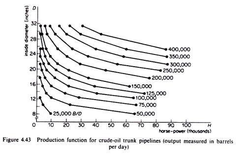
To illustrate the engineering method we will use L. Cookenboo’s study of the costs of operation of crude-oil trunk-lines. The first stage in the engineering method involves the estimation of the production function, that is, the technical relation between inputs and output. In the case of crude-oil trunk-lines output (X) was measured as barrels of crude oil per day. The main inputs in a pipeline system are ‘pipe diameter’, ‘horse-power of pumps’, ‘number of pumping stations’. Cookenboo estimated from engineering information the production function

X = (0-01046)^{-1/2 735.} H^0.37.D^1.73

Where X = barrels per day (the study was restricted to outputs ranging between 25,000 and 400,000 barrels per day)

H = horse-power

D = pipe diameter

The production function is homogeneous of degree 21, that is, the returns to scale are approximately equal to 2, implying that an increase in factor inputs by k per cent leads to an increase of output by 2k per cent. The input ‘number of pumping stations’, did not lend itself readily to a priori engineering estimation, and Cookenboo used for this input actual (historical) costs obtained from a pipeline company (after adjusting them for abnormal weather conditions prevailing during the construction of the pumping stations).

The production function relating X, H and D will depend on several factors such as the density of the crude oil carried through the pipes, the wall thickness of pipe used, and so forth. Cookenboo estimated his ‘engineering production function’ for the typical ‘Mid-Continent’ crude oil, and for wall thickness of ¼ inch pipe throughout the length of pipes (allowing 5 per cent terrain variation, and assuming no influence of gravity on flow of crude oil).

The above production function was computed by the use of a hydraulic formula for computing horse-powers for various volumes of liquid flow in pipes (adjusted with appropriate constants for the crude oil of Mid-Continent type). The estimated engineer­ing production function is shown in figure 4.43 (reproduced from Cookenboo’s work).

The second stage in the engineering method is the estimation of the cost curves from the technical information provided by the engineering production function. From the production function it is seen that a given level of output can be technically produced with various combinations of the D and H inputs.

In order to compute the long-run cost curve Cookenboo proceeded as follows. For each level of output he estimated the total cost of all possible combinations of H and D, and he chose the least expensive of these combinations as the optimum one for that level of output. The long-run cost curve was then formed by the least-cost combinations of inputs for the production of each level of output included in his study.

The total cost (for each level of output) includes three items, the costs of D, the costs of H, and ‘other costs’:

The costs of pipe diameter (D):

These include the cost of raw materials (steel, valves, corrosion protective, and so forth) and the labour costs of laying 1000 miles of pipe (this being the unit length of piping of ¼ inch wall).

The costs of horse-power (H):

These are the annual expenditures for electric power, labour and maintenance required to operate the pumping stations. Cookenboo included in this category the initial cost of pumping stations (costs of raw materials and labour costs).

Other costs:

These include the initial costs of storing-tank capacity, surveying the right- of-way, damages to terrain crossed, a communications system, and the expenses of a central office force. Cookenboo assumes that these costs are proportional to output (or to the length of pipes), with the exception of the last item (expenses of the central office force), which, however, he considers as unimportant:

There are no significant per-barrel costs of a pipe line which change with length. The only such costs are those of a central office force; these are inconsequential in relation to total. Hence, it is possible to state that (other) costs per barrel-mile for a 1000 mile trunk line are representative of costs per barrel-mile of any trunk line.

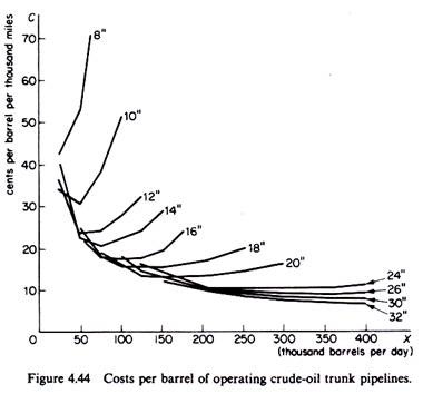
The derived long-run average-cost curve from the engineering production function is shown in figure 4.44 (based on Cookenboo’s work).

From his study Cookenboo concluded that the LR costs fall continuously over the range of output covered by his study. It should be noted that engineering cost studies are mainly concerned with the produc­tion costs and pay too little attention to the distribution (selling) and other administra­tive-managerial expenses. Given their nature, their findings are not surprising and cannot seriously challenge the U-shaped LR curve of the traditional theory. The existence of technical economies in large-scale plants has not been questioned.

Indeed, by their design large-scale plants have a lower unit cost, otherwise firms would not be interested in switching to such production techniques as their market increased; they would rather prefer to expand by duplicating smaller-size plants with whose operations their labour force (and their administrative staff) is familiar. What has been questioned is the existence of managerial diseconomies at large scales of output. And engineering cost studies are not very well suited for providing decisive evidence about the existence of such disecono­mies.

Engineering costs are probably the closest approximation to the economist’s produc­tion costs, since they avoid the problems of changing technology (by concentrating on a given ‘state of arts’) and of changing factor prices (by using current price quotations furnished by suppliers). Furthermore, by their nature, they provide ex ante information about the cost-output relation, as economic theory- requires. However, engineering costs give inadequate information about managerial costs and hence are poor approxi­mations to the total LAC of economic theory.

Another shortcoming of engineering cost studies is the underestimation of costs of large-scale plants obtained from extension of the results of the studies to levels of output outside their range. Usually engineering cost studies are based on a small-scale pilot plant. Engineers next project the input-output relations derived from the pilot plant to full-scale (large) production plants. It has often been found that the extension of the existing engineering systems to larger ranges of output levels grossly underestimates the costs of full-scale, large-size operations.

Finally, engineering cost studies are applicable to operations which lend themselves readily to engineering analysis. This is the reason why such studies have been found useful in estimating the cost functions of oil-refining, chemical industrial processes, nuclear-power generation. However, the technical laws underlying the transformation of inputs into outputs are not known with the desired detail for most of the manu­facturing industry, where, as a consequence, the engineering technique cannot be applied.

D. Statistical Production Function:

Another source of evidence about the returns to scale are the statistical studies of production functions. Most of these studies show constant returns to scale, from which it is inferred that the costs are constant, at least over certain ranges of scale. Like the statistical cost functions, statistical production functions have been attacked on various grounds. Their discussion goes beyond the scope of this book. The interested reader is referred to A. A. Walters’s article Econometric Production and Cost Functions’, Econometrica (1963).

E. The ‘Survivor technique’:

This technique has been developed by George Stigler. It is based on the Darwinian doctrine of the survival of the fittest.

The method implies that the firms with the lowest costs will survive through time:

(The basic postulate of the survivor technique) is that competition of different sizes of firms sifts out the more efficient enterprises.

Therefore by examining the development of the size of firms in an industry at different periods of time one can infer what is the shape of costs in that industry. Presumably, the survivor technique traces out the long-run cost curve, since it examines the develop­ment over time of firms operating at different scales of output.

In applying the survivor technique firms or plants in an industry are classified into groups by size, and the share of each group in the market output is calculated over time. If the share of a given group (class) falls, the conclusion is that this size is relatively inefficient, that is, it has high costs (decreasing returns). The criterion for the classifica­tion of firms into groups is usually the number of employees or the capacity of firms (as a percentage of the total output of the industry).

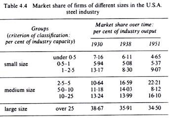
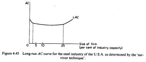
To illustrate the application of the survivor technique we present below the results of Stigler’s study of the economies of scale of the steel industry of the U.S.A. The firms have been grouped into seven classes according to their percentage market share.

From the data shown in table 4.4 Stigler concluded that during the two decades covered by his study there has been a continuous decline in the share of the small and the large firms in the steel industry of the U.S.A. Thus Stigler concluded that the small and the large firms are inefficient (have high costs). The medium-size firms increased or held their market share, so they constitute, according to Stigler, the optimum firm size for the steel industry in the U.S.A.

These findings suggest that the long-run cost curve of the steel industry has a con­siderable flat stretch (figure 4.45):

Over a wide range of outputs there is no evidence of net economies or diseconomies of scale.

The survivor technique, although attractive for its simplicity, suffers from serious limitations. Its validity rests on the following assumptions, which are rarely fulfilled in the real world.

It assumes that:

(a) The firms pursue the same objectives;

(b) The firms operate in similar environments so that they do not have locational (or other) advantages;

(c) Prices of factors and technology are not changing, since such changes might well be expected to lead to changes in the optimum plant size;

(d) The firms operate in a very competitive market structure, that is, there are no barriers to entry or collusive agree­ments, since under such conditions inefficient (high-cost) firms would probably survive for long periods of time.

Even if conducted with the greatest care and in conditions where the above assump­tions are fulfilled, the survivor technique indicates only the broad shape of the long-run cost curve, but does not show the actual magnitude of the economies or diseconomies of scale.

Another shortcoming of the survivor technique is that it cannot explain cases where the size distribution of firms remains constant over time. If the share of the various plant sizes does not change over time, this does not necessarily imply that all scales of plant are equally efficient. The size distribution of firms does not depend only on costs. Changes in technology and factor prices, entry barriers, collusive practices, objectives of firms and other factors as well as costs should be taken into account when analyzing the size distribution of firms over time.