The Traditional Theory of Costs (With Diagram)

Traditional theory distinguishes between the short run and the long run. The short run is the period during which some factors) is fixed; usually capital equipment and entrepreneurship are considered as fixed in the short run.

The long run is the period over which all factors become variable.

A. Short-Run Costs of the Traditional Theory:

In the traditional theory of the firm total costs are split into two groups total fixed costs and total variable costs:

TC = TFC + TVC

The fixed costs include:

(a) Salaries of administrative staff

(b) Depreciation (wear and tear) of machinery

(c) Expenses for building depreciation and repairs

(d) Expenses for land maintenance and depreciation (if any).

Another element that may be treated in the same way as fixed costs is the normal profit, which is a lump sum including a percentage return on fixed capital and allowance for risk.

The variable costs include:

(a) The raw materials

(b) The cost of direct labour

(c) The running expenses of fixed capital, such as fuel, ordinary repairs and routine maintenance.

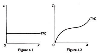
The total fixed cost is graphically denoted by a straight line parallel to the output axis (figure 4.1). The total variable cost in the traditional theory of the firm has broadly an inverse-S shape (figure 4.2) which reflects the law of variable proportions. According to this law, at the initial stages of production with a given plant, as more of the variable factors) is employed, its productivity increases and the average variable cost falls.

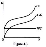
This continues until the optimal combination of the fixed and variable factors is reached. Beyond this point as increased quantities of the variable factors(s) are combined with the fixed factors) the productivity of the variable factors) declines (and the A VC rises). By adding the TFC and TVC we obtain the TC of the firm (figure 4.3). From the total-cost curves we obtain average-cost curves.

The average fixed cost is found by dividing TFC by the level of output:

AFC = TFC / X

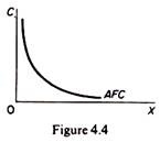
Graphically the AFC is a rectangular hyperbola, showing at all its points the same magnitude, that is, the level of TFC (figure 4.4).

The average variable cost is similarly obtained by dividing the TVC with the corresponding level of output:

AVC = TVC / X

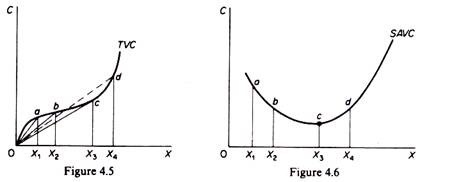
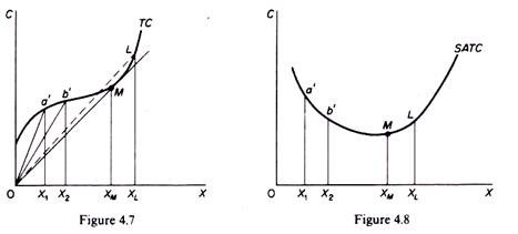
Graphically the A VC at each level of output is derived from the slope of a line drawn from the origin to the point on the TVC curve corresponding to the particular level of output. For example, in figure 4.5 the AVC at X₁ is the slope of the ray 0a, the A VC at X₂ is the slope of the ray Ob, and so on. It is clear from figure 4.5 that the slope of a ray through the origin declines continuously until the ray becomes tangent to the TVC curve at c. To the right of this point the slope of rays through the origin starts increasing. Thus the SA VC curve falls initially as the productivity of the variable factors) increases, reaches a minimum when the plant is operated optimally (with the optimal combination of fixed and variable factors), and rises beyond that point (figure 4.6).

The ATC is obtained by dividing the TC by the corresponding level of output:

ATC = TC / X = TFC + TVC / X = AFC + AVC

Graphically the ATC curve is derived in the same way as the SAVC. The ATC at any level of output is the slope of the straight line from the origin to the point on the TC curve corresponding to that particular level of output (figure 4.7). The shape of the A TC is similar to that of the AVC (both being U-shaped). Initially the ATC declines, it reaches a minimum at the level of optimal operation of the plant (X_M) and subsequently rises again (figure 4.8).

The U shape of both the AVC and the ATC reflects the law of variable proportions or law of eventually decreasing returns to the variable factor(s) of production. The marginal cost is defined as the change in TC which results from a unit change in output. Mathematically the marginal cost is the first derivative of the TC function. Denoting total cost by C and output by X we have

MC = ∂C / ∂X

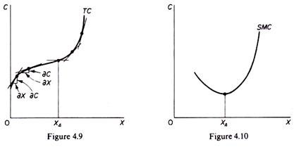
Graphically the MC is the slope of the TC curve (which of course is the same at any point as the slope of the TVC). The slope of a curve at any one of its points is the slope of the tangent at that point. With an inverse-S shape of the TC (and TVC) the MC curve will be U-shaped. In figure 4.9 we observe that the slope of the tangent to the total-cost curve declines gradually, until it becomes parallel to the X-axis (with its slope being equal to zero at this point), and then starts rising. Accordingly we picture the MC curve in figure 4.10 as U-shaped.

In summary: the traditional theory of costs postulates that in the short run the cost curves (AVC, ATC and MC) is U-shaped, reflecting the law of variable proportions. In the short run with a fixed plant there is a phase of increasing productivity (falling unit costs) and a phase of decreasing productivity (increasing unit costs) of the variable factor(s).

Between these two phases of plant operation there is a single point at which unit costs are at a minimum. When this point on the SATC is reached the plant is utilized optimally, that is, with the optimal combination (proportions) of fixed and variable factors.

The relationship between ATC and AVC:

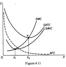
The AVC is a part of the ATC, given ATC = AFC + AVC. Both AVC and ATC are U-shaped, reflecting the law of variable proportions. However, the minimum point of the ATC occurs to the right of the minimum point of the AVC (figure 4.11). This is due to the fact that ATC includes AFC, and the latter falls continuously with increases in output.

After the AVC has reached its lowest point and starts rising, its rise is over a certain range offset by the fall in the AFC, so that the ATC continues to fall (over that range) despite the increase in AVC. However, the rise in AVC eventually becomes greater than the fall in the AFC so that the A TC starts increasing. The A VC approaches the A TC asymptotically as X increases.

In figure 4.11 the minimum AVC is reached at X₁ while the ATC is at its minimum at X₂. Between X₁ and X₂ the fall in AFC more than offsets the rise in AVC so that the ATC continues to fall. Beyond X₂ the increase in AVC is not offset by the fall in AFC, so that ATC rises.

The relationship between MC and ATC:

The MC cuts the ATC and the AVC at their lowest points. We will establish this relation only for the ATC and MC, but the relation between MC and AVC can be established on the same lines of reasoning.

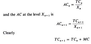
We said that the MC is the change in the TC for producing an extra unit of output. Assume that we start from a level of n units of output. If we increase the output by one unit the MC is the change in total cost resulting from the production of the (n + l)^th unit.

The AC at each level of output is found by dividing TC by X. Thus the AC at the level of X_n is

Thus:

(a) If the MC of the (n + 1)^th unit is less than AC_n (the AC of the previous n units) the AC _n+1 will be smaller than the AC_n.

(b) If the MC of the (n + 1)^th unit is higher than AC_n (the AC of the previous n units) the AC_n+1 will be higher than the AC_n.

So long as the MC lies below the AC curve, it pulls the latter downwards; when the MC rises above the AC, it pulls the latter upwards. In figure 4.11 to the left of a the MC lies below the AC curve, and hence the latter falls downwards. To the right of a the MC curve lie above the AC curve, so that AC rises. It follows that at point a, where the inter­section of the MC and AC occurs, the AC has reached its minimum level.

B. Long-Run Costs of the Traditional Theory: The ‘Envelope’ Curve:

In the long run all factors are assumed to become variable. We said that the long-run cost curve is a planning curve, in the sense that it is a guide to the entrepreneur in his decision to plan the future expansion of his output. The long-run average-cost curve is derived from short-run cost curves. Each point on the LAC corresponds to a point on a short-run cost curve, which is tangent to the LAC at that point. Let us examine in detail how the LAC is derived from the SRC curves.

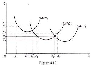
Assume, as a first approximation, that the available technology to the firm at a particular point of time includes three methods of production, each with a different plant size: a small plant, medium plant and large plant. The small plant operates with costs denoted by the curve SAC₁, the medium-size plant operates with the costs on SAC₂ and the large-size plant gives rise to the costs shown on SAC₃ (figure 4.12). If the firm plans to produce output X₃ it will choose the small plant. If it plans to produce X₂ it will choose the medium plant. If it wishes to produce X₁ it will choose the large- size plant.

If the firm starts with the small plant and its demand gradually increases, it will produce at lower costs (up to level X’₁). Beyond that point costs start increasing. If its demand reaches the level X”₁ the firm can either continue to produce with the small plant or it can install the medium-size plant. The decision at this point depends not on costs but on the firm’s expectations about its future demand. If the firm expects that the demand will expand further than X”₁ it will install the medium plant, because with this plant outputs larger than X’₁ are produced with a lower cost.

Similar con­siderations hold for the decision of the firm when it reaches the level X”₂. If it expects its demand to stay constant at this level, the firm will not install the large plant, given that it involves a larger investment which is profitable only if demand expands beyond X”₂. For example, the level of output X₃ is produced at a cost c₃ with the large plant, while it costs c’₂ if produced with the medium-size plant (c’₂ > c₃).

Now if we relax the assumption of the existence of only three plants and assume that the available technology includes many plant sizes, each suitable for a certain level of output, the points of intersection of consecutive plants (which are the crucial points for the decision of whether to switch to a larger plant) are more numerous. In the limit, if we assume that there is a very large number (infinite number) of plants, we obtain a continuous curve, which is the planning LAC curve of the firm.

Each point of this curve shows the minimum (optimal) cost for producing the corresponding level of output. The LAC curve is the locus of points denoting the least cost of producing the corresponding output. It is a planning curve because on the basis of this curve the firm decides what plant to set up in order to produce optimally (at minimum cost) the expected level of output.

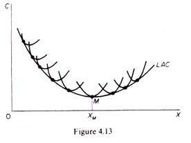
The firm chooses the short-run plant which allows it to produce the anticipated (in the long run) output at the least possible cost. In the traditional theory of the firm the LAC curve is U-shaped and it is often called the ‘envelope curve’ because it ‘en­velopes’ the SRC curves (figure 4.13).

Let us examine the U shape of the LAC. This shape reflects the laws of returns to scale. According to these laws the unit costs of production decrease as plant size increases, due to the economies of scale which the larger plant sizes make possible. The traditional theory of the firm assumes that economies of scale exist only up to a certain size of plant, which is known as the optimum plant size, because with this plant size all possible economies of scale are fully exploited.

If the plant increases further than this optimum size there are diseconomies of scale, arising from managerial inefficiencies. It is argued that management becomes highly complex, managers are overworked and the decision-making process becomes less efficient. The turning-up of the LAC curve is due to managerial diseconomies of scale, since the technical diseconomies can be avoided by duplicating the optimum technical plant size.

A serious implicit assumption of the traditional U-shaped cost curves is that each plant size is designed to produce optimally a single level of output (e.g. 1000 units of X). Any departure from that X, no matter how small (e.g. an increase by 1 unit of X) leads to increased costs. The plant is completely inflexible. There is no reserve capacity, not even to meet seasonal variations in demand.

As a consequence of this assumption the LAC curve ‘envelopes’ the SRAC. Each point of the LAC is a point of tangency with the corresponding SRAC curve. The point of tangency occurs to the falling part of the SRAC curves for points lying to the left of the minimum point of the LAC since the slope of the LAC is negative up to M (figure 4.13) the slope of the SRMC curves must also be negative, since at the point of their tangency the two curves have the same slope.

The point of tangency for outputs larger than X_M occurs to the rising part of the SRAC curves since the LAC rises, the SAC must rise at the point of their tangency with the LAC. Only at the minimum point M of the LAC is the corresponding SAC also at a minimum. Thus at the falling part of the LAC the plants are not worked to full capacity; to the rising part of the LAC the plants are overworked; only at the minimum point M is the (short-run) plant optimally employed.

We stress once more the optimality implied by the LAC planning curve each point represents the least unit-cost for producing the corresponding level of output. Any point above the LAC is inefficient in that it shows a higher cost for producing the correspon­ding level of output. Any point below the LAC is economically desirable because it implies a lower unit-cost, but it is not attainable in the current state of technology and with the prevailing market prices of factors of production. (Recall that each cost curve is drawn under a ceteris paribus clause, which implies given state of technology and given factor prices.)

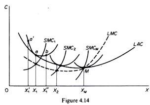
The long-run marginal cost is derived from the SRMC curves, but does not ‘en­velope’ them. The LRMC is formed from points of intersection of the SRMC curves with vertical lines (to the X-axis) drawn from the points of tangency of the corresponding SAC curves and the LRA cost curve (figure 4.14). The LMC must be equal to the SMC for the output at which the corresponding SAC is tangent to the LAC. For levels of X to the left of tangency a the SAC > LAC.

At the point of tangency SAC = LAC. As we move from point a’ to a, we actually move from a position of inequality of SRAC and LRAC to a position of equality. Hence the change in total cost (i.e. the MC) must be smaller for the short-run curve than for the long-run curve. Thus LMC > SMC to the left of a. For an increase in output beyond X, (e.g. X’₁) the SAC > LAC. That is, we move from the position a of equality of the two costs to the position b where SAC is greater than LAC. Hence the addition to total cost (= MC) must be larger for the short-run curve than for the long-run curve. Thus LMC < SMC to the right of a.

Since to the left of a, LMC > SMC, and to the right of a, LMC < SMC, it follows that at a, LMC – SMC. If we draw a vertical line from a to the X-axis the point at which it intersects the SMC (point A for SAC₁) is a point of the LMC.

If we repeat this procedure for all points of tangency of SRAC and LAC curves to the left of the minimum point of the LAC, we obtain points of the section of the LMC which lies below the LAC. At the minimum point M the LMC intersects the LAC. To the right of M the LMC lies above the LAC curve. At point M we have

SAC_M = SMC_M = LAC = LMC

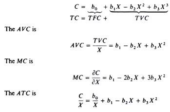
There are various mathematical forms which give rise to U-shaped unit cost curves. The simplest total cost function which would incorporate the law of variable pro­portions is the cubic polynomial

The TC curve is roughly S-shaped , while the ATC, the AVC and the MC are all U-shaped; the MC curve intersects the other two curves at their minimum points (figure 4.11).