Cobb-Douglas Production Function | Econometrics

In this article we will discuss about the Cobb-Douglas production function.

The production function is defined as technical relationship between physical quantity of inputs and physical quantity of output of any sector, agricultural sector or industrial sector.

This functional relationship can be specified as follows:

Y = f (X₁, X₂, X₃…………… X_n)

Where

Y = Physical quantity of output and

X₁, X₂, X₃……………. X_n = Physical quantities of inputs employed.

If X₁ is labour and X₂ is capital in the function then the following economic relationships will be obtained.

Marginal Product of Labour [MPX₁]

MPX₁ = ΔY/ ΔX₁, whose value is always supposed to be positive. The Marginal Product of Labour goes on declining with the increase in X₁.

The Marginal Product of Capital.

MPX₂ = ΔY/ΔX₂, whose value is also always supposed to be positive. The Marginal Product of Capital also goes on declining with the increase in X₂.

The elasticity of output with respect to labour or capital is the ratio of the marginal product of the concerned input [MPX₁ or MPX₂] to the average product of the same [APX₁ or APX₂].

The elasticity of output with respect to [e_y.x1] will be estimated as follows:

e_Y.X1 = ΔY/ΔX₁.X₁/Y

1] If it’s value is less than unity, then the proportionate change in output will be lower than the proportionate change in input X₁: 2] If it is more than unity, then the proportionate change in output will be higher than the proportionate change in input X₁ :3] If it is unity, then the proportionate change in output will be equal to the proportionate change in input X₁.

The above statements imply that:

[1] MPX₁ < APX₁ and APX₁ declines with an increase in labour input.

[2] MPX₁ > APX₁ and APX₁ increases with an increase in labour input.

[3] MPX₁ = APX₁ and APX₁ will be constant with an increase in labour input.

The elasticity of output with respect to capital [e_y.x2] will also be estimated as follows:

e_Y.X2= ΔY/ΔX₂.X₂/Y

1] If it’s value is less than unity, then the proportionate change in output will be lower than the proportionate change in input X₂:2] If it is more than unity, then the proportionate change in output will be higher than the proportionate change in input X₂:3] If it is unity, then the proportionate change in the output will be equal to the proportionate change in input X₂.

The above statements imply that:

[1] MPX₂ < APX₂ and APX₂ declines with an increase in capital input

[2] MPX₂ > APX₂ and APX₂ increases with an increase in capital input

[3] MPX₂ = APX₂ and APX₂ will be constant with an increase in capital input

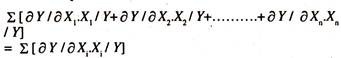
The returns to scale will be estimated to know the responsiveness of output to the changes in all the inputs simultaneously.

This will be estimated by taking the sum of the elasticities of output with respect to different inputs included in the production function as shown below:

 

 

 

If the sum of the elasticities is more than unity, then there will be increasing returns to scale; [Non-linear homogeneous production function]; If the sum is less than unity, then there will be decreasing returns to scale [Non-linear homogeneous production function]; If the sum of the elasticities is equal to unity, then there will be constant returns to scale [Linear homogeneous production function]

Linear Production Function:

On the assumption of a linear relationship between the output and the set of inputs, the following relationship [model] will be specified:

Y = b₀+ b₁ X₁+ b₂ X₂+……….. + b_nX_n+ error………….. (94)

The partial derivative of Y with respect to X₁ is

∂Y/∂X₁ = b₁, Which is constant marginal product of labour [MPX₁], all else equal.

The partial derivative of Y with respect to X₂ is

∂Y/∂X₂ = b₂ , Which is constant marginal product of capital [MPX₂], all else equal.

Similarly the partial derivatives of output with respect to other inputs will also be estimated.

The elasticity of output with respect to X₁ will be estimated as follows:

e_Y.X1= [∂Y / ∂X_i.X_i / Y]

= b₁*Y/X₁

The value of elasticity of Y with respect of X₁ goes on changing with the change in Y or X₁ , if the individual values are considered. Therefore it is referred to as variable elasticity.

Similarly the elasticity of output with respect to X₂ will be estimated as follows:

e_Y.X1= ∂Y/ ∂ X₂.X₂/ Y = b₂X₂/ Y.

The value of elasticity of Y with respect to X₂ goes on changing with the change in Y or X₂.Therefore it is referred to as variable elasticity, if the individual values are considered The elasticities of output with respect to different inputs [X₁ and X₂] in the linear production function will be inversely related to the increase in X₁ or X₂, all else equal.

In empirical production function studies the elasticities of output with respect to different inputs will be evaluated at the mean values of Y,X₁ and X₂. Therefore they will be referred to as the average elasticities.

If the e_Y.X1 > 1, then the proportionate change in Y will be higher than the proportionate change in X₁. If the e_Y.X1 < 1, then the proportionate change in Y will be less than the proportionate change in X₁. If the e_Y.X1 = 1, then the proportionate change in Y will be equal to the proportionate change in X₁

From the linear production function, the estimate of returns to scale [Responsiveness of output to the changes in all the inputs] can be obtained by taking the sum of the elasticities [evaluated at the mean value] as shown below:

 

If it is more than 1, then there will be increasing returns to scale. If it is less than 1, then there will be decreasing returns to scale. If it is equal to 1, then there will be constant returns to scale.

But the choice of the linear production function depends on economic, statistical and econometric criteria. If the linear function fitted to the cross-section or time series observations is not found to be appropriate, then other form of equation such as power function will be attempted.

Cobb-Douglas Production Function:

The Specification of a power function, which is well- known as Cobb-Douglas Production Function [double log or log linear or constant elasticity model], will be as follows:

Y = b₀X₁^b1 X₂^b2………….X_n^bn (95) 

The partial derivative of Y with respect to X₁, keeping other variables constant

∂Y/∂X₁ = b₁ [b₀ X₁^b1-1 X₂^b2 ……………X_n^bn]

= b₁ [b₀ X₁^b1 X₂^b2X_n^bn] X₁

= b₁ [Y] X₁^-1

= b₁Y / X₁, is known as marginal product of labour. This is inversely related to increase in labour input, all else equal. Therefore, the marginal product of labour goes on diminishing with the increase in labour input.

The partial derivative of Y with respect to X₂, keeping other variables constant

∂Y/∂X₂ = b₂ [b₀ X₁^b1 X₂^b2-1 ……………X_n^bn]

= b₂ [b₀ X₁^b1 X₂^b2………..X_n^bn] X₂^-1

= b₂ [Y] X₂^-1

= b₂ Y/X₂ , is known as marginal product of capital.

This is inversely related to increase in capital. Therefore, the marginal product of capital also [or any input] goes on diminishing with the increase in capital input all else equal.

Thus, the marginal products of labour and capital will be in line with the theory according to which, if the variable input labour or capital is successively employed in the operation of production, all else equal, the marginal product of that variable input goes on diminishing.

In order to examine whether the production function curve [emerged out of the power production function or Cobb-Douglas production function] has concavity to the input [If labour input is considered] axis, it is necessary to consider the second derivative [derivative of the first derivative] of the function

Fist derivate of the function with respect to labour input

 

 

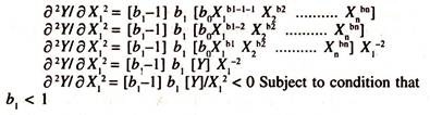
Thus if ∂ Y/ ∂ X₁ < 1 and ∂²Y/∂X₁² < 0, then the power function [Cobb Douglas function] will have concavity to labour input axis implying that marginal product of labour diminishes with increase in Labour.

The regression coefficients of different inputs in the Cobb Douglas production function function will be constant partial elasticities as shown below:

 

 

 

 

 

 

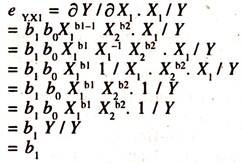
Thus, b₁ is the constant partial elasticity of output with respect to input labour.

The elasticity of output with respect to capital will also be constant as shown below:

 

 

 

 

 

 

 

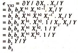
Thus, b₂ is also constant elasticity of output with respect to input capital.

Returns to Scale [Homogeneous Production Function]:

The estimate of returns to scale can be estimated from the Cobb-Douglas production function by taking the summation of the regression coefficients [constant elasticities] of various inputs. In other words it is the sum of elasticities of output with respect to different inputs. [In case of two inputs X₁ and X₂]

i.e., ∑ [b₁ + b₂]

=∑[∂ Y/∂ X_i. X_i/Y]

If the sum is more than 1, then there will be increasing returns to scale [Non Linear Homogeneous Production Function]. If the sum is less than 1, then there will be decreasing returns to scale [Non Linear Homogeneous Production Function], If the sum is equal to 1, then there will be constant returns to scale [Linear Homogenous Production Function],

Returns to Variable [Non-Homogeneous Production Function]:

It should be noted that if the elasticity of output with respect to labour is less than unity [b₁ < 1], all else equal, then there will be decreasing returns to labour variable [non linear non-homogeneous production function].

If it is more than unity [b₁> 1], all else equal, then there will be increasing returns to labour variable [Non Linear Non-Homogeneous Production Function], If it is equal to unity [b₁= 1], all else equal, then there will be constant returns to labour variable [Linear Non- Homogeneous Production Function].

Thus, the advantage of estimating the Cobb-Douglas production function is that the nature of returns to variable [labour or capital] and returns to scale can simultaneously be assessed. Since the above function is related to a multiple linear regression model, there will be multi-collinearity problem between labour and capital.

Therefore, the problem of multi-collinearity needs to be reduced by adopting different methods. Per capita [Ratio of output to labour = Output per labour unit = Y/X₁ ; Ratio of Capital to labour = Capital per labour unit = X₂/X₁] specification is one of the remedial measures to over come the problem of multicollinearity between X₁ and X₂.

[Y/X₁] = b₀ [X₂/X₁]^b1 ………….(96)

Where

Y = Output

X₁= Labour

X₂ = Capital

Y/X₁ = Per Capita Output [Output per unit of labour]

X₂/X₁ = Per Capita Capital [output per unit of capital]

For the purpose of estimation, the above function is transformed into a log-linear model as shown below:

 

 

 

 

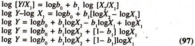
Where

b₂ = 1 – b₁

1 = b₁+ b₂ [Restricted to unity implying Constant returns to scale or linear homogeneous production function]

The derivative of log Y with respect of log X₂ is the elasticity of output with respect to capital [b₁] and the elasticity of output with respect to X₁ is 1 – b₁. It should be noted that the sum of the elasticities of output with respect to capital and labour will be unity evincing the presence of constant returns to Scale [known as linear homogeneous production function] If, the sum of these two elasticities in the multiple log-linear regression model [∑(b₁ +b₂) in log Y = b₀ + b₁ log X₁ + b₂ log X₂ or Y = b₀ X₁^b1 X₂^b2 ] is equal to unity, then the per capita specification may be preferred.

If the sum of the elasticities of output with respect to labour and capital is more than unity or less than unity, the fitting of per capita specification to the data restricts to constant returns to scale, which undermines the presence of both increasing or decreasing returns to scale. In empirical studies more than two inputs are used in the production function analysis to capture the impact of these inputs on output in terms of marginal products, elasticities, returns to scale, returns to variable etc.,

The Cobb-Douglas production function, which can be especified either in log- linear form or power function form, is widely used to fit the production functions in agricultural and industrial sectors by ordinary least squares method. One of the limitations of Cobb- Douglas production function is that the elasticity of substitution between two inputs will all the time be unity, which is not true always across units, firms or industries.

In view of this limitation other form of production function namely Constant- Elasticity of Substitution Production Function [CESPF] is considered. It will be appropriate to see the unitary elasticity of substitution in Cobb-Douglas production function.

An isoquant [Isoproduct] gives equal product with different combinations of inputs. In order to increase the quantity of one input, the quantity of other input has to be given up. The ratio of the change in capital to change in labour is known as marginal rate of technical substitution [MRTS] i.e.,

MRTS = -ΔX₂/ΔX₁

Marginal rate of technical substitution is also equal to the ratio of the marginal product of labour to marginal product of capital i.e.,

-ΔX₂/ΔX₁ = MPX₁/MPX₂

This can be proved from the total differentiation. The change in total production is equal to the sum of marginal product of labour times the change in labour + marginal product of capital times the change in capital

Δ Y = MPX₁* ΔX₁ + MPX₂ * ΔX₂

On isoproduct curve, production doesn’t change.

Therefore, ΔY = 0 [zero].

This can be explained as follows:

 

 

 

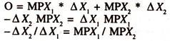
Thus, the ratio of marginal product of labour [MPX₁] to marginal product of capital [MPX₂] is the marginal rate of technical substitution. The size of elasticity of substitution, which is free from the units of measurement, [e_s = σ ] is unity in Cobb-Donglas Production Function.

This can be proved as follows:

 

 

 

 

 

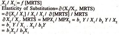
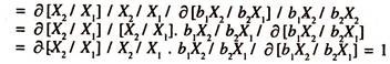
The Specification of the above function will be as follows:

 

 

For the purpose of estimation by ordinary least squares method logarithms have to be taken on both sides of the equation.

log[X₂/ X₁] = logb₀ + σ log [b₁X₂/ b₂X₁] ……………………..(99)

The derivative of log [X₂ /X₁] with respect to log [b₁X/b₂X₁] is σ, whose value will always be unity though constant. This is a restrictive assumption of Cobb-Douglas production function. In view of this, the CES production function is preferred in empirical production function studies. The estimation of the elasticity of substitution between inputs in the CES Production Function.

Estimation of Law of Variable Proportions:

The empirical validity law of variable proportions, the behaviour of the production of specific crop [P] to the changes in single variable, land [L], all else equal, can be studied by fitting the following form of quadratic equation without intercept

P = β₁ L+ β₂L²

This equation is mathematically derived for empirical estimation of the law of variable proportions as follows:

Production is equal to area under crop [L] and productivity of land [LP]

P = L*LP…………….. [1]

An inverse linear relationship between productivity of land and area under crop [farm size] can be expressed as follows

LP = β₁ – β₂ L ……………. [2]

Substituting the equation [2] into equation[l] the following quadratic equation will be obtained:

P = L [β₁ – β₂L] = β₁L – β₂L²…………… [3].

Thus the empirical estimation of the law of variable proportions is based on equation [3].

If the intercept is included in the equation [3] the estimable form of equation [quadratic production function] with an intercept will be as follows:

P = β₀+ β₁L- β₂ L²

The marginal product of land [derivative of P with respect to L]

dP/dL =β₁ – 2 β₂ [L] goes on diminishing with the increase in farm size

By setting the first derivative to zero ,the farm size can be determined to know the maximum Production of the crop with a sufficient condition that the second derivative must be < 0

dP/dL = 0

β₁-2β₂[L] = 0

Solving for L

β₁ =2 β₂ [L]

β₁ / 2 β₂ = [L]

The second derivative = d²P/dL² = – 2 β ₂ < 0

With the help of the elasticity of production with respect to land [e], the nature of returns to variable [ constant/ increasing/diminishing returns to variable] can be assessed

e = dP/dL*L/P

= β₁-2 β₂ [L] *L/P

If e < 1 then there will be diminishing returns to variable

If e > 1 then there will be increasing returns to variable

If e = 1 then there will be constant returns to variable

Production Function – Estimates of Economic Relationships:

The time series data given in Table 10.1 on output, labour and capital for the Indian manufacturing sector are considered to estimate the linear and Cobb-Douglas production functions.

The regression results of the linear production function [Table 10.2] show that the regression coefficient of labor is negatively insignificant. Here one has to be very cautious in explaining the results as the regression coefficient of labour is supposed to be positive. The regression coefficient of capital [marginal product of capital] is significantly positive.

The elasticity of production with respect to capital [estimated at mean values of Y and X₂ : 3.0926 (22302.81/71297.25)] is close to unity, That is 0.96741. The data transformed into log Y, log X₁and log X₂] given in table 10.3 are used to estimate log linear production function.

The results of the log linear production function or Cobb Douglas production function [Table 10.4] show that the regression coefficient of labour [elasticity of production with respect to labour] is insignificant with erroneous sign which could be due to the problem of multicollinearily between log X₁ and log X₂ or inappropriate labour variable.

The regression coefficient of capital, which is elasticity of output with respect to capital, is significantly positive showing that a one percent increase in capital would increase the output by 0.974 percent, all else equal. Since the regression coefficient of labour is insignificant, the estimate of returns to scale will be calculated by taking the value of regression coefficient of capital.

In order to avoid the problem of multicolliearity between labour and capital, the series on per capita variables are generated and given in table 10.5. The results of the production function based on per capita specification [restricted production function] [Table 10.6] show that the regression coefficient of [Y/X₁] is significantly positive showing that a one percent increase in [X₂/X₁] leads to increase the [Y/X₁] by 0.965 percent.

In order to estimate the linear and Cobb-Douglas production function the cross-sectional farm data [Table 10.7] are also considered.

The results of the linear production function fitted to the cross sectional farm data [Table 10.8] show that the regression coefficients of labour and capital [marginal products of labour and capital respectively] are significantly positive and less than unity.

The output elasticity of labour [estimated at the mean values of Y and X₁:0.017965*1268.643/76.50=0.297924] is 0.297 showing that a one percent increase in labour leads to increase the paddy output by 0.297 percent, all else equal.

The output elasticity of capital [estimated at the mean values of Y and X₂: 0.017210*2977.143/76:50=0.66976] is 0.669&. showing that a one percent increase in capital leads to increase the paddy output by 0.6698 percent, all else equal.

The estimate of returns to scale, sum of the output elasticities of labour and capital [0.29710 + 0.669 = 0.966] is 0.966 showing that there are decreasing returns to scale. In order to estimate the Cobb-Douglas production function the cross sectional farm data [at a point of time] are transformed into natural log form. The series are furnished in table 10.9

The regression results [Table 10.10] show that the coefficients of log X₁ and log X₂ [direct output elasticities of labour and capital] are significantly positive but less than unity as observed in the case of the linear production function.

The sum of the elasticities, estimate of returns to scale, is 0.909 showing that there are decreasing returns to scale. The marginal products of labour [0.0225= 0.356467*59.6425/ 941.278] and capital [0.01478= 0.553903*59.6425/ 2237.035878] estimated at the geometric mean values of Y,X₁ and X₂ are positive and less than unity.

It should be noted that the economic relationships in the estimated production function such as marginal products, output elasticities and returns to scale are found to be identical both in the linear and log linear [Cobb Douglas] production functions so far as the signs and magnitudes are concerned. The concern is the choice of the production function that depends on economic, statistical and econometric criteria.

Unitary Elasticity of Substitution in Cobb-Douglas Production Function:

The following cross sectional farm data [Table 10.11] are considered to illustrate that the elasticity of substitution between two inputs, X₁ and X₂, is, all the time, unity in cobb-douglas production function. (X₂/X₁) = constant [MRTS] σ = log (X₂/X₁) = constant + σ log[MRTS]), though constant.

In cobb-douglas production function MRTS is equal to MPX₁/MPX₂. In order to prove this the Cobb Douglas production function is estimated. The results of the same are presented in table 10.12 to generate the required series for estimating the elasticity of substitution between two inputs. The series generated the are furnished in table 10.13

The regression results based on log(X₂/X₁) = constant + σ log(MRTS) are presented in table 10.14

The regression results show that the constant elasticity of (X2/X1) with respect to MRTS [log (X₆)] is found to.be unity. As this is restrictive value of elasticity of substitution in Cobb Douglas production function, the CES production function is being considered in empirical studies to test whether the numerical value of elasticity of substitution is different from unity or not.