Price Competition with Differentiated Product | Oligopoly Models

The below mentioned article provides quick notes on price competition with differentiated product.

Oligopolistic markets can have some degree of product differentiation.

Market shares are determined not just by prices, but also by durability, design and performance of each firm’s product. It is quite natural for firms to compete by choosing prices rather than quantities. To see how price competition can work with differentiated products, we will go through the following example.

Suppose, each duopolist has a fixed cost of £20 but zero variable cost and that they face the same demand curves.

Firm 1’s Demand Curve : Q₁ = 12 – 2P₁ + P₂…….. (4)

Firm 2’s Demand Curve: Q₂ = 12 – 2P₂ + P………… (5)

where P₁ and P₂ are the prices charged by Firms 1 and 2 respectively, and Q₁ and Q₂ are the quantities they sell. It may be noted that the quantity each firm can sell increases when its competitor charges higher price and decreases when the firm raises its own price.

If both firms set their prices at the same time, we can use the Cournot model to determine equilibrium. Each firm will choose its own price, taking the competitor’s price as fixed.

We consider the case of Firm 1. Its profit is π₁ – P₁Q₁ minus the fixed cost of £20.

Substituting Q₁ from the demand curve of equation (4), we get:

π₁ – P₁Q₁ – 20

= 12P₁ – 2P₁² + P₂P₁ – 20.

At what price P is this profit maximised? To answer this question, we need to know P₂, which Firm 1 assumes as fixed. However, whatever price Firm 2 charges, Firm l’s profit is maximised when dπ/dP₁ = 0.

Taking P₂ as fixed, Firm 1’s profit-maximising price is given by:

dπ/dP₁ = 12 – AP₁ + P₂ = 0.

From this equation, we can find the reaction curve of Firm 1:

Reaction Curve of Firm 1: P₁ = 3 + 1/4 P₂.

This indicates to Firm 1 what price to set, given that Firm 2 has set its price P₂.

Similarly we can find the Firm 2’s reaction curve as follows:

Reaction Curve of Firm 2: P₂ = 3 +1/4 p₁.

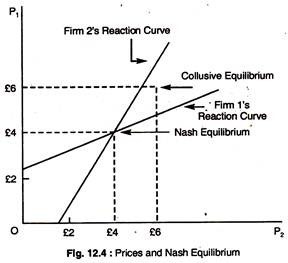
These reaction curves are drawn in Fig. 12.4. The Nash Equilibrium is at the point where the two reaction curves intersect, where each firm charges a price of £4, and earns a profit of £12. At this point, since each firm is doing the best it can, given the price of its competitor neither firm has an incentive to change its price.

Also shown in the diagram is the collusive equilibrium which they can set, if they cooperate. In this case price is £6.