Kinked Demand Curve Model of Oligopoly (With Diagram)

In this article we will discuss about:- 1. Assumptions of the Kinked Demand Curve Model 2. Why the Kink in the Demand Curve? 3. Analysis of the Kinked Demand Curve Model.

Assumptions of the Kinked Demand Curve Model:

This model was developed independently by Prof. Paul M. Sweezy on the one hand and Profs. R. C. Hall and C. J. Hitch on the other hand.

The assumptions of this model are:

(i) There are only a few firms in an oligopolistic market.

(ii) The firms are producing close-substitute products.

(iii) The quality of the products remains constant and the firms do not spend on advertising.

(iv) A set of prices of the product has already been determined and these prices prevail in the market at present.

(v) Each firm believes that if it reduces the price of its product, the rival firms would follow suit, but if it increases the price, then the rivals would not follow it, they would simply keep their prices unchanged. We shall see presently that, because of this asymmetric reaction pattern of the rivals, the demand curve of each firm would have a kink at the prevailing price of its product.

Why the Kink in the Demand Curve?

In Fig. 14.18 we have drawn two negatively sloped straight line demand curves, viz., dd’ and DD’. Of these two curves, dd’ is more flat than DD’. Now, when one particular firm in the industry changes the price of its product, all other firms keeping their prices constant, the firm’s demand curve will be rela­tively flatter like dd’, i.e., the magnitude of the change in the demand for its product as its price changes would be relatively larger.

This is because, as the firm reduces or increases the price of its product, the prices of the products of other firms remaining constant, the product of the firm becomes relatively cheaper or dearer, respec­tively, than those of the other firms.

On the other hand, if a particular firm in the industry changes the price of its product, and following this, all other firms also change their prices in the same direction, and, say by the same proportion, for the sake of simplicity, then the firm’s demand curve would be relatively more steep like DD’.

This is because, in this case, as the firm decreases or increases the price, its product does not become neither relatively cheaper nor dearer. Therefore, now its demand curve would be less elastic, or more steep, than dd’—now the demand curve would be like DD’.

Let us suppose that initially the price of the product of the firm is p₁ or Op₁ and the demand for the product is q₁ or Oq₁ If the firm now increases its price from p₁, the rival firms would keep their prices unchanged according to assumption (v) of this model.

In this case, the firm’s demand would decrease along the segment Rd of the relatively more elastic demand curve dd’. On the other hand, if it goes on decreasing its price from p₁, its rivals also would be decreasing their prices according to assumption (v). In this case, the quantity demanded of the firm’s product will increase along the segment RD’ of the relatively steeper demand curve DD’.

Therefore, at the price p₁, the firm’s demand curve would be dRD’. Obviously, because of assumption (v), the segment dR of this demand curve would be more flat or more elastic than the segment RD’ (and the segment RD’ would be more steep or less elastic than the segment dR).

As a result, there would be a kink at the prevailing price p₁, or, at the point R on the firm’s demand curve d RD’, i.e., the demand curve in this model would be a kinked demand curve.

Analysis of the Kinked Demand Curve Model:

In the oligopoly model under discussion, the properties of the kinked demand curve as well as its significance are especially discussed. In the first place, as the demand curve or the average revenue (AR) curve of the firm has a kink, its MR curve cannot be obtained as a continuous curve. We may, therefore, begin with the properties of the MR curve of the kinked demand curve with the help of Fig. 14.19.

The kinked demand curve of the firm in this Fig. is dRD’. There is a kink at the point R (p₁, q₁) on this curve, because the curve consists of a segment dR of the relatively flatter curve dd’ and another segment RD’ of the relatively steeper curve DD’.

Therefore, in the case of the kinked demand curve dRD’, the firm’s MR curve, up to q = q₁, would consist of the MR curve dM associated with the dR segment of the kinked demand curve and for q > q₁, the MR curve would be the segment NB associated with the segment RD’ of the demand curve.

We have obtained above that the firm’s MR curve for its kinked demand curve would consist of two parts, viz., the segments dM and NB, and there would be a vertical gap between the points M and N at q = q₁.

This implies that as the firm’s output goes on increasing up to q₁, its MR would go on decreasing along the segment dM up to the amount Mq₁ and if the firm’s output increases even by an infinitesimally small quantity at q = q₁, its MR would fall to Nq₁, and, thereafter, as q increases, MR would decrease along the segment NB.

In other words, there would be no MR value between Mq₁ and Nq₁, i.e., the dotted segment MN is the discontinuity in the firm’s MR curve. We may also say that at the point R on the dR segment of the kinked demand curve, the firm’s MR would be Mq₁ and, at the point R on the RD’ segment of the demand curve, MR would be Nq₁.

We may now easily see that the numerical coefficient of elasticity of demand (e₁) at the point R on the demand curve segment dR is different from the coefficient (e₂) at the point R on the demand curve segment RD’, and the larger the difference between e₁ and e₂, the larger would be the length of the discontinuity of the MR curve at the output q₁.

As we know, at any point R (p₁, q₁) on the firm’s demand curve in Fig. 14.19, numerical coefficient (e) of price- elasticity of demand is

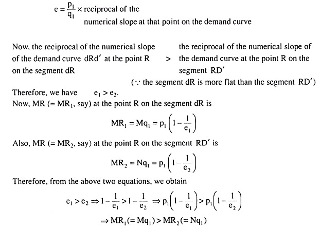
That is, at the point of kink, R, on the demand curve dRD’, or at q = q₁, we have two different values (e₁ and e₂) of e, and that is why at q = q₁, we obtain two different values (MR! and MR₂) of MR and two different parts of the MR curve. The vertical gap between the two parts of the MR curve at q = q₁ is Mq₁ – Nq₁ = MN.

It follows from the above discussion that the larger the difference between e, and e₂, i.e., the more flat the segment dR would be than the segment RD’, i.e., the more prominent the kink would be at the point R, the larger would be the value of MR₁ than that of MR₂ and the larger would be the discontinuity in the MR curve at q = q₁.

Second, in the model under discussion, the prices of the products are given initially, and a relation between these prices has been established already. The model does not explain how these prices have been determined.

But there is a good chance that the price of the product of a firm would be consistent with its goal of profit maximisation. For example, in Fig. 14.20, the firm’s demand curve is dRD’ and the associated MR curve is MR₁—the discontinuity or the vertical gap between the two parts of the MR₁curve is MN.

Now, if the marginal cost (MC₁) curve of the firm passes through this gap of MN, then the firm’s price-output combination R(p₁, q₁) is consistent with profit maximisation although here, at q = q₁, we have MR (= Mq₁) > MC (= Lq₁), and not MR = MC.

Here we see that at q < q₁ MR > MC, making the firm increase its output to reach the profit-maximising point. Now, as q increases and becomes equal to q₁, then also we have MR > MC. But if the firm increases q beyond q₁, MR becomes less than MC (MR < MC), i.e., from the production and sale of the marginal unit of its output, the firm now would incur a loss.

Therefore, it would not produce more than q₁, and its profit would be maximum at q = q₁, in spite of the fact that at q = q₁, we have MR > MC, and not MR = MC.

Third, although the assumption (v) of the model regarding the reaction pattern of the rival firms may explain the kink in the firm’s demand curve, it cannot explain how the price of the firm’s product, or, for that matter, the prices of the rivals’ products, are determined.

However, the reac­tion pattern of the rivals, as given by assumption (v), is able to explain why the prices would not tend to change, i.e., why they would be sticky, once they get determined.

For example, if, in Fig. 14.20, the firm’s quantity sold increases from q₁ to q₂, it would not be inclined to change the assumption regarding the reac­tion pattern of the rivals, for its conception about the rivals’ reactions, is, by no means, dependent on its quantity sold.

Therefore, it would regard the increase in quantity sold, or an increase in the demand for its product, as caused by a rightward shift in its demand curve—it would think that its demand curve has shifted to the right from dRD’ to dR’D”.

We may note here that although the demand curve has shifted to the right, it has kept the price of its product unchanged, resulting not necessarily in the unfulfilment of its profit maximising goal.

In Fig. 14.20, we have assumed that the two curves, viz., dRD’ and dR’D”, are iso-elastic (2.8.2g), and the MC₁ curve passes also through the discontinuity (M₁N₁) of the MR₂ curve which is the marginal curve for the demand curve dR’D”. Therefore, here the firm is able to maximise its profit at the same price p₁ = R’q₂ = Rq₁.

Fourth, in the model under discussion, the firm may not have to change the price of its product, even if its cost of production rises. For example, let us suppose that initially the firm’s AR and MR curves are dRD’ and MR₁, and the MC, curve is the firm’s MC curve.

In this case, the firm’s profit would be maximised if it sells q₁ of output at the price of p₁. Now, if the firm’s cost position changes resulting in an upward shift in its MC curve from MC₁ to MC₂, and if the MC₂ curve also, like MC₁, passes through the discontinuity (MN) of its MR curve, then the firm would not have to change the price of its product in order to earn the maximum profit.

It would be able to maximise profit if it, like the previous case, sells of output at the price of p₁.

If the cost of production rises along with a shift in the demand curve, then also, profit maximisation may not require the firm to change the price of its product. For example, in Fig. 14.20, let us suppose that the firm’s AR, MR and MC curves are, respectively, dRD’, MR₁and MC₁, In this case, the firm’s profit-maximising price-output combination would be R (p₁ q₁).

Now, if the firm’s MC curve rises to MC₂ along with a rightward shift in its demand curve to dR’D”, then also the firm would not be required to change the price of its product if the MC₂ curve passes through both the discontinuities, MN and M₁N₁, of its dRD’ and dR’D” curves.

It would still be able to earn the maximum profit at the price pi; but now its quantity of output produced and sold would be q₂; that is, now the firm’s price-output combination would be obtained at the point R’ (p₁, q₂).

On the basis of the above discussion, we may conclude that in the kinked demand curve model of oligopoly, the firm would not consider it profitable or rational to change the prevail­ing price of its product because of the assumption (v) relating to the reaction pattern of its rivals.

[This assumption states, that if a particular firm increases the price of its product, its rivals will not increase theirs, but if it reduces the price, they will promptly reduce their prices.] We have seen that, because of these reactions, the demand curve of each oligopolistic firm will be kinked, and the MR curve of this demand curve will have two separate segments, and there will be a vertical gap between them.

However, it is not that the firm’s goal of profit maximisation can never be achieved because of the existence of this vertical gap. Even when the firm’s demand increases, i.e., its demand curve shifts to the right and/or its MC curve shifts upwards, it is not impossible for it to achieve profit maximisation at the prevailing price.

There­fore, although the kinked demand curve model cannot explain the process of price deter­mination, it can well explain why the prices are sticky in an oligopolistic market.