Bertrand developed his duopoly model in 1883. His model differs from Cournot’s in that he assumes that each firm expects that the rival will keep its price constant, irrespective of its own decision about pricing.
Thus each firm is faced by the same market demand, and aims at the maximization of its own profit on the assumption that the price of the competitor will remain constant.
The model may be presented with the analytical tools of the reaction functions of the duopolists.
In Bertrand’s model the reaction curves are derived from isoprofit maps which are convex to the axes, on which we now measure the prices of the duopolists. Each isoprofit curve for firm A shows the same level of profit which would accrue to A from various levels of prices charged by this firm and its rival.
ADVERTISEMENTS:
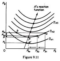
The isoprofit curve for A is convex to its price axis (PA). This shape shows the fact that firm A must lower its price up to a certain level (point e in figure 9.11) to meet the cutting of price of its competitor, in order to maintain the level of its profits at ΠA2. However, after that price level has been reached and if B continues to cut its price, firm A will be unable to retain its profits, even if it keeps its own price unchanged (at PAe). If, for example, firm B cuts its price at PB, firm A will find itself at a lower isoprofit curve (ΠA1) which shows lower profits. The reduction of profits of A is due to the fall in price, and the increase in output beyond the optimal level of utilization of the plant with the consequent increase in costs. Clearly the lower the isoprofit curve, the lower the level of profits.
To summaries for any price charged by firm B there will be a unique price of firm A which maximizes the latter’s profit. This unique profit-maximizing price is determined at the lowest point on the highest attainable isoprofit curve of A. The minimum points of the isoprofit curves lie to the right of each other, reflecting the fact that as firm A moves to a higher level of profit, it gains some of the customers of B when the latter increases its price, even if A also raises its price.
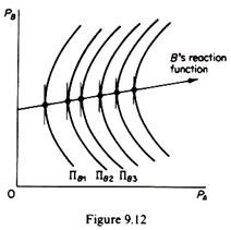
If we join the lowest points of the successive isoprofit curves we obtain the reaction curve (or conjectural variation) of firm A: this is the locus of points of maximum profits that A can attain by charging a certain price, given the price of its rival. The reaction curve of firm B may be derived in a similar way, by joining the lowest points of its isoprofit curves (figure 9.12).

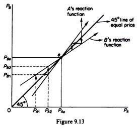
Firm A will react to this decision of its rival by charging a higher price PA2. Firm B will react by increasing its price, and so on, until point e is reached, when the market will be in equilibrium. The same equilibrium will be reached if firms started by charging a price higher than PAe or PBe a competitive price cut would take place which would drive both prices down to their equilibrium level PAe and PBe.
Note that Bertrand’s model does not lead to the maximization of the industry (joint) profit, due to the fact that firms behave naively, by always assuming that their rival will keep its price fixed, and they never learn from past experience which showed that the rival did not in fact keep its price constant. The industry profit could be increased if firms recognized their past mistakes and abandoned the Bertrand pattern of behaviour (figure 9.14).
If firms moved on any point between c and d on the Edge-worth contract curve (which is the locus of points of tangency of the isoprofit curves of the competitors) one or both firms would have higher profits, and hence industry profits would be higher. At point c firm B would retain the same profit (B6) as at point e, while A would move to a higher profit level (A9). At point d firm A would have the same profit (A5) as at the Bertrand equilibrium e, but firm B would move to a higher isoprofit curve (B10). Finally, at any point between c and d (e.g. at f) both firms would realize higher profits (A7 and Bs) as compared to those attained at Bertrand’s solution (A7 > As and Bs > B6).
ADVERTISEMENTS:
Bertrand’s model may be criticised on the same grounds as Cournot’s model:
The behavioural pattern emerging from Bertrand’s assumption is naive: firms never learn from past experience.
Each firm maximises its own profit, but the industry (joint) profits are not maximized.
The equilibrium price will be the competitive price. (In the example of costless mineral-water production, the price in Bertrand’s model would fall to zero. If production is not costless, then price would fall to the level which would cover the costs of the duopolists inclusive of a normal profit.)
The model is ‘closed’-does not allow entry.
The interesting feature of both Cournot’s and Bertrand’s models is that the limit of duopoly is pure competition. Neither model refutes the other. Each is consistent and is based on different behavioural assumptions. We may say that Bertrand’s assumption (about the fixity of price of the rival) is more realistic, in view of the observed preoccupation of firms with keeping their prices constant (except in cost inflation situations).
Furthermore, Bertrand’s model focused attention on price setting as the main decision of the firm. The serious limitations of both models are the naive behavioural pattern of rivals; the failure to deal with entry; the failure to incorporate other variables in the model, such as advertising and other selling activities, location of the plant, and changes in the product.
Product differentiation and selling activities are the two main weapons of non-price competition, which is a main form of competition in the real business world; both models do not define the length of the adjustment process. Although dealing in terms of ‘time periods,’ their approach is basically static; both models assume that the market demand is known with accuracy; both models are based on individual demand curves which are located by making the convenient assumption of constant reaction curves of the competing firms.
ADVERTISEMENTS:
Having discussed the classical duopoly models of Cournot and Bertrand, we proceed with the development of the traditional models of non-collusive oligopoly, which apply to market structures with a few firms conscious of their interdependence. It is worth while pointing out, however, that both Cournot’s and Bertrand’s models can be extended to markets in which the number of firms is greater than two.


