Effectiveness of Monetary Policy: IS-LM Curves, Economist’s Views and Limitations

The question of effectiveness of monetary policy has three aspects- technical, theoretical and practical, (a) Technically the IS and LM curves serve as analytical tools for explaining the effectiveness of monetary policy. (b) Theoretically relativeness of monetary policy in comparison with fiscal policy is discussed by examining Keynesian and monetarist view on the subject, (c) Practically, various limitations or the factors disturbing the effectiveness of monetary policy in the real world are discussed.

(a) The IS-LM Curves and Effectiveness of Monetary Policy:

The IS and LM curves are the powerful analytical tools to explain the effectiveness of the monetary policy. With the help of these curves, it can be shown under what conditions the monetary policy is effective in changing the level of income in the economy. The IS curve slopes downwards because as income increases, saving also increases and rate of interest falls.

Each point on the IS curve is a point of equilibrium between saving and investment, indicating equilibrium in the product market. The LM curve slopes upwards because as income increases, rate of interest also rises because of a rise in the demand for money.

Each point on the LM curve is a point of equilibrium in the money market. The intersection of die IS and LM curves determine the equilibrium levels of income and rate of interest.

Effectiveness of monetary policy is a function of the slopes of the IS and LM curves. Flatter the IS curves (i.e, more interest elastic the investment) and/or steeper the LM curve (i.e, lesser the speculative demand for idle money and greater the tendency to spend), more effective will be monetary policy. Various cases of effectiveness of monetary policy have been explained below with the help of Figure 2.

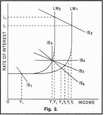
(i) When the IS curve (IS₁) cuts the LM curve in the Keynesian liquidity trap range (i.e., horizontal portion of the LM curve), an increase in the money supply (from LM₀ to LM₁) is completely ineffective. In this case, the speculative demand for money is maximum, velocity of money is minimum, rate of interest remains unchanged at the lowest level Oi₀, investment is not encouraged and there is no increase in the income level which remains at OY₀.

(ii) When the IS curve (IS₂) cuts the LM curve in the classical range (i.e. vertical portion of the LM curve), an increase in money supply (LM₀ to LM₁) is most effective. In this case, the speculative demand for money is zero, velocity of money is maximum, rate of interest falls (from Oi₂ to Oi₁), investment increases and as a result income increases (from OY₂ to OY₆).

(iii) When the IS curve (IS₃) cuts the LM curve in the intermediate range (upward sloping portion of the LM curve), an increase in money supply will increase the income level, but not as much as in the case of classical range when the LM curve is vertical. In the classical case, the rate of interest falls so much as to absorb the whole additional money supply into the transactions demand, thus leading to increase in investment. In the intermediate range, a part of the increase in the money supply will be held for speculative motive. As a result, investment will not increase to the extent as .in the classical case and income will increase by lesser amount (from OY₁ to OY₄)

(iv) An increase in money supply from (LM₀ to LM₁) is completely effective when investment is perfectly interest elastic (i.e. horizontal IS₄). Income increase from OY₁ to OY₅.

(v) An increase in money supply (from LM₀ to LM₁) is completely ineffective when investment is perfectly interest inelastic (i.e., vertical IS₅). Income does not increase at all and remains at OY₁ level.

(vi) An increase in money supply (from LM₀ to LM₁) is more effective when investment is relatively elastic (flatter IS₃). Income increases from OY₁ to OY₄.

(vii) An increase in money supply (from LM₀ to LM₁) is less effective when investment is relatively inelastic (i.e. steeper IS₆). Income increase from OY₁ to OY₃.

(b) Keynesians and Monetarists on Effectiveness of Monetary Policy:

Economists are divided on the question of effectiveness of monetary policy. Two extremely opposite views have been presented by the Keynesians and the monetarists regarding the effectiveness of monetary and fiscal policies.

Keynesian View:

Keynesians are the modern followers of J.M. Keynes and have reformulated his original ideas.

Keynesian view is based on the assumptions:

(a) That the capitalist economy is inherently unstable;

(b) That this instability is primarily due to the variability of investment spending and produces violent business cycles; and

(c) That such an economy needs to be stabilised, can be stabilised and should be stabilised by appropriate monetary and fiscal policies.

Keynesians believe that the economy operates under liquidity trap range (horizontal LM curve), so that only fiscal policy (i.e., changes in the IS curve), can influence the level of income, output and employment. The IS curve is considered to be vertical or interest inelastic.

General economic condition of the economy resembles that of depression; prices, income level, rate of interest and velocity of money are very low, and speculative demand for money is very high.

Keynesians believe that fiscal policy is superior and more effective than monetary policy.

Fiscal policy is more effective because it affects aggregate demand:

(a) Directly through changes in the government expenditure, and

(b) Indirectly through changes in taxes and transfer payments which cause changes in consumption.

On the other hand; monetary policy is less reliable because of the following reasons:

(i) Monetary policy is less predictive in its results. During depression, when interest rates are already very low, people have a tendency to hold money rather than purchase bonds. Thus, increases in money supply may be offset by decreases in velocity of money. Thus, according to the equation of exchange, MV = PT = Y, the net change in MV, and hence in PT = Y, is unpredictable.

(ii) Monetary policy will be effective if (a) increase in money supply leads to significant fall in interest rate, and (b) fall in interest rate leads to significant increase in investment. Symbolically, ∆M → ∆i → ∆I → ∆ AD. But in depression, interest rates are already low. Moreover, demand for business loans is very small because of the low profit expectations.

Thus, since both the links, i.e., ∆M → ∆i and ∆i → ∆I are weak, the effect of changes in money supply (∆M) on aggregate demand (AD) will be insignificant and, therefore, monetary policy will be ineffective during depression.

(iii) In the short-run, the price level and the level of nominal national product are determined by a number of factors and monetary policy is only one among them. Other factors are fiscal policy, changes in autonomous consumption, inflationary expectations and shifts in aggregate supply due to increases in wages or raw material prices.

(iv) There is a role for monetary policy in inflation. Monetary authority can decrease the supply of money and cause interest rate to rise. While financial institutions cannot be forced to lend excess reserves, they can be forced to meet reserve requirements.

But, here also Keynesians are doubtful about the efficacy of monetary policy because of its effect on velocity of money. When money supply is increased, velocity of money falls, and when money supply is decreased, velocity of money rises.

Figure 3 shows the ineffectiveness of the monetary policy and effectiveness of fiscal policy during depression. According to Keynesians, during depression, the IS₀ curve is vertical, indicating that net investment is not responsive to changes in the interest rate. The vertical ISO curve intersects the LM curve in the Keynesian liquidity trap range.

In this range, an increase in money supply from LM₀ to LM₁ has no effect on income (OY₀) and rate of interest (Oi₀). Since interest rate is unaffected and investment is unresponsive to changes in rate of interest, income remains unchanged and monetary policy is rendered ineffective.

On the other hand, the fiscal policy involving an increase in the government expenditure shifts the IS₀ curve to IS₁. As a result, income increases from OY₀ to OY₁. As long as the economy is in the liquidity trap, increases in government expenditure will produce multiple increase in income, output and employment because interest rate does not rise and there is no crowding out of private investment. Hence, fiscal policy is fully effective.

Monetarist View:

Monetarists are the modern non-Keynesian economists with classical roots. They trace their lineage to classical and neo-classical economists, and from them to Milton Friedman and others.

Monetarist view is based on the fundamental assumptions:

(a) That the capitalist economy is inherently stable;

(b) That much of the instability actually experienced since World War II has been the result of active fiscal and monetary policies;

(c) That there is no need to stabilise the economy; and

(d) That if there is need, it cannot be done because stabilisation policies are more likely to increase than to decrease instability.

Monetarists believe that the economy operates under the classical range (vertical LM curve) so that only monetary policy (i.e., changes in the LM curve) can affect the level of income, output and employment. The IS curve normally slopes downward. General economic condition of the economy resembles that of inflation; prices, income level, rate of interest, and velocity of money are very high, and speculative demand for money is at a minimum.

Monetarists do not consider fiscal policy to be very effective in affecting the macro variables. They maintain that, other things- being constant, changes in government expenditure can cause multiplier effects. But, the ‘other things’ (e.g., the rate of interest) are not likely to remain constant. If government expenditures are financed by borrowing from the public, interest rates will rise and some private investment will be crowded out.

On the other hand, monetary policy can prove more effective in influencing macro variables especially in the short period. The monetarists provide historical evidence in favour of the monetary policy.

Milton Friedman and Anna Jacobson Schwartz have concluded from the monetary history of the United States that- (a) Changes in the behaviour of the money stock have been closely associated with changes in economic activity, money income and prices, (b) The interrelation between monetary and economic change has been highly stable, (c) Monetary changes have often had an independent origin; they have not been simply a reflection of changes in economic activity.

While the monetarists prefer monetary policy, their true position is that the discretionary monetary policy may have destablising effects on the economy. The time lag between the application of the monetary policy and its effects on economic variables is so unpredictable and political pressures on the government are so great that the monetary policy will destabilize the economy.

Therefore the monetarists prefer a monetary rule reflecting the economy’s natural growth rate of output to discretionary monetary policy. The government should pursue a fixed monetary rate known to everyone instead of using its discretion.

Figure 4 shows the monetarist view, i.e., the effectiveness of monetary policy and ineffectiveness of fiscal policy. The monetarists deal with the other extreme, i.e., the vertical (classical) range of the LM₀ curve. An increase in the government expenditure shifts IS₀ to IS₁.

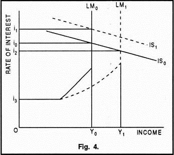
As a result, the interest rate rises room Oi₀ to Oi₁ and the increase in the government expenditure is completely offset by a decrease in private investment. Thus, income remains at OY₀ level. On the other hand, given IS₀ curve, an expansionary policy will shift LM₀ to LM₁.

This will reduce the rate of interest from Oi₀ to Oi₂, encourage investment and thus increase income level from OY₀ to OY₁. Thus according to monetarists, fiscal policy is ineffective and monetary policy is effective in influencing the income level of the economy.

Conclusion:

Keynesian and monetarist views on effectiveness of monetary and fiscal policy along with their implications are summarised below:

(i) The extreme Keynesian and monetarist views are partial, one-sided and contain half-truths. Both the approaches deal with a particular phase of trade cycle in a capitalist economy.

(ii) Keynesian view is more suitable during the phase of depression; it is useful in forecasting changes in income level when the economy is experiencing depression.

(iii) Monetarist view works in the inflationary phase; it helps in forecasting change in income level in an inflationary situation.

(iv) The moderate view is that more of monetarism and less of Keynesianism during inflation and more of Keynesianism and less of monetarism during deflation will help in promoting economic growth with stability in developed countries.

(v) However, all the three approaches (i.e., extreme Keynesian, extreme monetarist and the moderate approaches) will not be of much help to the developing economies because these approaches mainly deal with the regulation of demand and supply of monetary factors, whereas the developing countries are facing the real problem of generation and allocation of physical factors.

(c) Limitations and Problems of Monetary Policy:

Monetary policy has been defined as a policy of the central bank to control the money supply for achieving the objectives of general economic policy. This implies that the problem of monetary policy is the determination of tire optimal quantity of money, or in dynamic conditions, the optimal rate of growth of the money stock.

But, in actual practice, it is difficult not only to define but also to determine the optimal money stock. In fact, monetary policy is much more than the simple determination of money stock.

In the real world, monetary policy faces a number of problems which reduce its scope and effectiveness:

1. Conflicting Goals:

It is difficult to define optimal money stock because the ultimate goals or objectives of monetary policy (such as, price stability, exchange stability, full employment, economic growth) may be in conflict. For example, the central bank reduces the growth rate of money supply to stabilise the price level.

But this slower rate of growth of money supply may increase unemployment rate and reduce the rate of economic growth. Similarly, a faster rate of growth of the money supply may reduce unemployment and increase the rate of economic growth, but on the other hand, may create disequilibrium in the balance of payments or generate intolerably high rate of inflation.

2. Lags in Monetary Policy:

Even if the goal variables, such as output, employment and prices, have been successfully determined, the appropriate monetary policy will be able to affect them only after a time lag. The changes in the monetary policy and the resultant changes in the aggregate spending are not directly linked.

The monetary policy influences the aggregate spending through three links, i.e., changes in the supply of money, cost of money (i.e., rate of interest) and availability of money.

These links may not be quickly responsive to changed monetary policy and may not produce quick changes in aggregate expenditure:

(a) Commercial banks may or may not adjust quickly to changes in the monetary policy and change the cost and availability of credit accordingly,

(b) Reduced rate of interest may influence the aggregate spending after some time because it takes time to plan and execute the investment projects,

(c) Changes in money supply may affect aggregate spending after a long period because in the short run the individuals and business firms may try to use their existing money balance more intensively.

Thus, it requires a long time for the monetary policy to have its effect on the level of demand and thus to achieve the desired objectives.

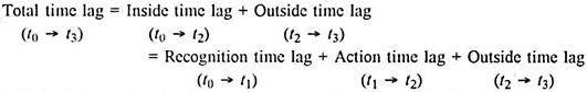
Time lags are of many types:

(i) Recognition Time Lag:

Before a policy is formulated, the policy makers need information on the current condition of the economy. The time required to gather information about the current state of the economy is called recognition time lag. They must know, for example, what is happening to the rate of capital formation, the unemployment rate etc.

Again, just one piece of information is not enough: there must be supporting evidences from several time series data covering same period of time. Thus, it takes time to obtain accurate information about the current problem of the economy. Suppose, the economy is experiencing recession, it takes t₀ to t₁ time to recognise this problem, then t₀ -> t₁ will be recognition time lag.

(ii) Action Time Lag:

Once the problem is recognised, it requires some time for the policy makers to suitably adjust or alter the policy. The time required between recognising an economic problem and putting the policy into effect is called action time lag.

Action time lag may be due to several reasons:

(a) Time is required to work out details of change in the policy and the administrative details to implement them,

(b) Sometimes, delay is caused by the controversy among the policy makers about the need for a change in the policy,

(c) Political pressures may also delay the policy change,

(d) Generally, the action time lag is shorter for the monetary policy and longer for fiscal policy.

Suppose, the time taken by policy maker to make necessary changes in the policy is from time t₁ to t₂ then t₁ → t₂ will be action time lag.

(iii) Inside Time Lag:

The sum of recognition time lag and action time lag is known as inside time lag. In other words, inside time lag = recognition time lag + action time lag. If recognition time lag is t₀ → t₁ and action time lag is t₁ → t₂ then inside time lag, i.e. t₀ → t₂ = t₀ → t₁ + t₁ → t₂. The length of inside time lag depends upon time required for data collection and its analysis, administrative delays, policy trade-offs and priorities, etc.

(iv) Outside Time Lag:

Once policy has been changed, it requires additional time for the policy to effect changes in aggregate spending. The time that elapses between the onset of policy and the results of that policy is called outside time lag or effect time lag. A change in the rate of growth of money supply, for example, takes time to work itself out and ultimately influence the economic activity in the economy.

The outside time lag depends upon the complex interrelationships in the working of the economy and, therefore, it is difficult to make an accurate estimate of its length. If the time period between the changes in the policy and the resultant changes in the economic activity is from t₂ to t₃, then the outside time lag will be t₂ → t₃.

To sum up:

3. Changes in Velocity of Money:

Changes in the velocity of money held by the public are another factor which restricts the effectiveness of the monetary policy. Tight monetary policy becomes ineffective in controlling inflation. The monetary authority can control the money supply and not the velocity of money.

Velocity of money can vary in a number of ways:

(i) Development of Nonbank Financial Intermediaries:

Growth of non-bank financial intermediaries since World War II has greatly restricted the role of monetary policy. Their activities are not under the control of central bank.

Nonbank financial intermediaries limit the effectiveness of monetary policy in two ways:

(a) In times of tight money policy, the nonbank financial intermediaries can sell government securities to holders of idle demand deposits in the commercial banks, and thus can activate the deposits and raise the velocity of money,

(b) By raising the interest rates during the tight money policy, the nonbank intermediaries can attract hitherto idle demand deposits away from the commercial banks and re-lend them. This also increases the velocity of money stock.

(ii) Portfolio Adjustment of Commercial Banks:

Commercial banks policy of portfolio adjustment can make the monetary policy ineffective. If these banks decide to meet the loan requirements of borrowers by selling government securities lying with them, this will increase the aggregate spending in the economy without any increase in the money supply. Under such conditions, velocity of money increases and the restrictive monetary policy becomes ineffective.

(iii) Intensive Use of Available Money Supply:

The private sector can render the restrictive monetary policy of the central bank ineffective by making a better and more effective use of existing money supply. Adoption of improved methods, such as collection of funds by sales finance companies, borrowing funds by companies from public by offering higher interest rates, etc., definitely increases the velocity of money in the economy and makes monetary policy ineffective.

4. Target Problem:

Target problem arises because the monetary policy cannot directly and quickly affect the ultimate objectives (e.g., exchange stability, price stability, full employment, etc.) through its instruments (e.g., bank rate, open market operations, reserve requirements; etc.).

Monetary policy, in order to be effective, must affect spending decisions. But the chain of causation from the starting of a policy action to its ultimate effect on aggregate demand is so complex and indirect that the effectiveness of the policy action becomes doubtful and unpredictable.

Therefore, the policy makers select some intermediate targets (such as, money supply, bank credit, interest rate) which are directly affected by the instruments of bank rate, open market operations, etc. In this way, by using the instruments to attain intermediate targets, the central bank hopes to achieve the ultimate objectives more effectively.

Intermediate targets or target variables or proxy variables for the ultimate goal variables are endogenous variables which the monetary authority influences in order to influence the ultimate variables in the desired manner.

A good intermediate target must satisfy the following conditions- (a) It should be closely related with the ultimate goal variables and its relation should be clearly understood and properly estimable, (b) It should be quickly influenced by policy instruments (c) Non-policy influences on it should be small as compared to the policy influences, (d) It should be easily observable or measurable without any time lag.

5. Indicator Problem:

Indicator problem arises because there is possibility that the intermediate target variables are influenced by some non-policy exogenous factors. In other words, it is possible that changes other than those induced by policy action may effect the target variables.

The policy makers, therefore, need some other variable, called monetary policy indicator to separate the policy induced effect from the non-policy induced effect and to adjust the policy accordingly.

In this sense, the indicator will be at least one step close to the monetary authorities than the target variable. The ideal indicator will be that which is influenced only by policy actions. Like the target variable, the indicator should be- (a) easily observable, with no time lag, (b) immediately influenced by the policy action, and (c) related to the target and the goal variable.