Effectiveness of Fiscal and Monetary Policy (With Diagram)

Let us make an in-depth study of the Effectiveness of Fiscal and Monetary Policy. After reading this article you will learn about: 1. Fiscal Policy 2. Monetary Policy 3. Interaction of Monetary and Fiscal Policies 4. The Monetary-Fiscal Policy Mix.

Fiscal Policy:

The size of the fiscal policy (FP) multiplier or the effectiveness of fiscal policy depends on whether FP change is initiated at a low or high level of output relative to full employment output.

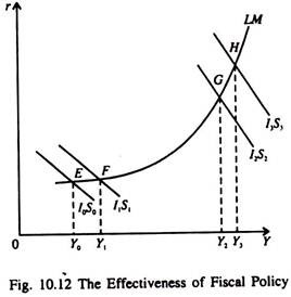
This point is illustrated in Fig. 10.12.

It shows differing effects on Y of a given IS shift, depending on where on the LM curve the policy actions start.

At the initial equilibrium Y₀, the LM curve is relatively flat, with almost zero slope (over the range AB). This gives a large FP multiplier nearly equal to that in SKM, without any adverse development in the money market. But at the initial equilibrium point with income Y₂ the LM curve is nearly vertical with a very high slope. In this case FP multiplier is very low, almost equal to zero as the LM curve becomes vertical.

The size of the FP (G or T) multiplier de­pends on the slope of the LM curve at the initial equilibrium point. A certain increase m G and shift in IS will lead to a large increase in Y if the economy starts from a situation of high unemployment and low interest rates.

But if G is increased in a situation where the economy is approaching full employment (with tight labour markets), Y will not increase much. In this case the sharp increase in r will cause investment to fall so much that it almost offsets the favourable effects of the increase in G.

Thus we see that the size of fiscal policy multiplier itself depends on the initial cyclical position of the economy.

Comparison of Effects of Changes in G and T:

It may apparently seem that the effects of equivalent fiscal policy changes in G or T on the levels Y will be the same.

But there are two major differences between the effects of these two types of fiscal policy (FP) changes:

(i) The composition of output:

Prima facie, expanding output by increasing G will also increase the government’s share of output. The increase in government purchases (G) increases the provision of public goods. But a tax cut shifts the initial stimulus to policy-induced increase in consumer spending raising the share of output of consumer goods in GDP.

(ii) The effect of saving:

It is also possible for consumers to save the additional disposable income in which case the S + T schedule will remain unchanged and there will be no effect on Y. This problem does not arise with changes in G. The reason is that the government can ensure that G changes by the desired (required) amount.

Thus the outcome of an increase in G on Y is more certain than that of a cut in T or an increase in transfer payments. Moreover, if tax cuts are of a temporary nature and are unlikely to affect the permanent income of the people tax cuts will raise saving temporarily rather than boost consumption permanently.

Therefore, a choice of which policy instrument to use to expand (or contract) output will in part depend on how the policy maker wants the composition of output to change.

Monetary Policy:

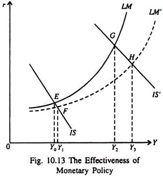
The effectiveness of monetary policy (MP) also varies with the cyclical position of the economy. As Fig. 10.13 shows, with a given slope of the IS curve, a given shift of the LM curve due to an increase in the money supply will have a stronger effect on Y when Y and r are high rather than when they are low.

Fig. 10.13 shows that MP is more effec­tive when the LM curve is vertical as rela­tively higher levels of r and Y, than when it is flat. So MP is most effective (and FP is most ineffective) when the economy is at a high r, Y level and is able to utilise almost its entire money supply to support financial transactions, that is, to support Y.

The effectiveness of the two policies depends on how they interact with each other. We may now discuss this issue to examine their relative effectiveness.

Interaction of Monetary and Fiscal Policies:

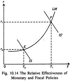
Fig 10.14 shows that the relative effective­ness of MP and FP depends on the shape of the LM curve and the initial state of the economy, i.e., whether it is in depression or is nearing full employment. If the economy is in the initial position such as r₁, Y₁, an expansion­ary MP shifting the LM curve to the right may have little effect on Y.

The reason is that at the initial value of r the additional money will be absorbed by speculative demand this will pre­vent r from falling further. So no stimulus is provided to investment. On the other hand at r₁, Y₁, a shift of the IS curve will be relatively effective in raising Y. The reason is that a marginal rise in r will release adequate funds from speculative balances to support an in­crease in Y.

The Monetary-Fiscal Policy Mix:

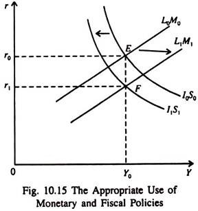
By making appropriate use of MP and FP instruments (policy variables) it is possible to achieve the best of both the worlds. The government can bring the desired changes in r and the composition of output without shifting the demand curve, that is, without changing Y (from the demand side Y= C + I + G) at a fixed price level. This point is illustrated in Fig. 10.15.

In Fig. 10.15 the level of output Y₀ yields virtual full employment at the exist­ing price level. However, the existing rate of interest (r₀) may be considered as too high. In such a situation it is possible for the government to reduce r by raising the tax total permanently by shifting the I₀S₀ to I₁S₁, and reducing consumption demand.

This could be offset by increasing money supply, lowering r and stimulating I, bringing the economy back to Y₀ — at the low rate of interest r₁. This shift in the monetary-fiscal policy mix tightening the fiscal screw and loosening the monetary belt has shifted the composition of the equilibrium Y₀.

With G fixed, C has been reduced and I increased. Thus FP and MP variables can be changed in opposite directions to alter the composition of demand without shifting the C + I + G schedule.

In short, FP is most effective when the economy is in deep depression — with interest rates low and unemployment high. But in an economy with a very high level of both capital and labour utilisation and high interest rates, the money supply will be the restraining factor and MP will be most effective.

Further Notes on Crowding-Out Effect:

Crowding-out effect refers to the possibility that an increase in one form of spending may cause another form to fall. Normally bond financing of budget deficit leads to ‘crowding- out’. This may happen in various ways. See Table 10.3.

1. Shortage of scarce resources and delays in private projects:

Let us suppose government spending on public works rises. This might use scarce resources, such as skilled engineers, diverting them from alternative investment projects which are thus delayed.

2. Tight monetary policy:

Alternatively, if increased demand (C + I + G) causes inflation this might lead to tighter monetary policy, thus cutting both C and / by raising r.

3. Loss of confidence among private investors due to growing volume of public debt:

Finally, if private investors are made nervous by increased debt, a rise in public works might scare-off private investment.

i. Full Crowding Out vs. Partial Crowding-Out:

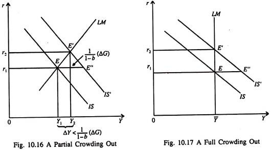
Full (total) crowding-out occurs if other spending falls by 100% of the rise in public works. Partial crowding-out occurs if other spending falls, but by less than the amount by which public spending rises.

A rise in G shifts the IS curve to the right and increases r along a given LM curve. This crowds out investment and partially offsets the favourable effects of the rise in G on Y. In Fig. 10.16 there is partial crowding-out and in Fig. 10.17 full crowding-out.