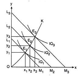
While deriving the expansion path of the firm from its production function:
q = f(x, y) [eqn. (8.21)]
if we assume that the firm uses the variable inputs X and Y along with some fixed inputs, then it should be understood that we are discussing the short run and in that case the firm’s expansion path, OK, as obtained in Fig. 8.14, would be a short-run expansion path.
Fig. 8. 14 The expansion path of a firm
ADVERTISEMENTS:
In the case of such an expansion path, the cost incurred by the firm for the two inputs, i.e., the cost as entered in the equation of the ICL, would be the firm’s total variable cost (TVC), and if we add the firm’s total fixed cost (TFC) to this TYC, we would obtain the firm’s short-run total cost (STC).
On the other hand, if we assume that the firm uses two variable inputs, X and Y, and no fixed inputs, then it should be understood that we are discussing the long run. In that case, the same expansion path, viz., OK, would be the firm’s long-run expansion path. In the case of such an expansion path, the level of cost that is entered in the equation of the ICL should be taken as the long-run total cost (LTC) of the firm.
Again, of the two inputs, X and Y, that are used by the firm, one, say X, is a variable input and the other, Y, is a fixed input, then also the expansion path derived from the production function would be a short-run expansion path.
ADVERTISEMENTS:
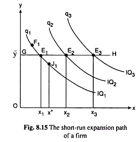
But, in this case, the expansion path would not be same as OK of Fig. 8.14. Rather it would be a horizontal straight line at the level of the fixed amount of input Y measured along the vertical axis. We have illustrated the derivation of such an expansion path in Fig. 8.15.
In this Fig., we have assumed that the quantity of input Y has been assumed to be fixed at y̅ in the short run. Therefore, in the short run, the firm would use varying quantities of the variable input X along with the given amount of the fixed input to expand its operations.
For example, if the firm intends to produce the output quantity of q1 on IQ1, it would be in cost-minimizing equilibrium at the point E1(x1, y̅).
ADVERTISEMENTS:
E1 is the cost-minimising point subject to q = q1, because at any other point on IQ1, say, at F1 to the northwest of E1, the required quantity of Y would be more than y̅, which is unavailable, or, at a point like J1 to the southeast of E1, the required quantity of Y would be less than y and that of X more than x1.
Consequently, at J1 the cost of output q1 would be higher than that at the point E1, because here the expenditure on Y being fixed at p1y̅, the expenditure on X would be larger than that at E (pXx* > pXx1).
Similarly, if the firm decides to expand and produce a higher q at q2 on IQ2, it would have to produce at the point E2(x2, y̅). For at E2, the cost would be minimum possible, since given
y = y, x = x2 is the minimum amount of X that would be required to produce q = q2.
In the same way, if the firm’s output is to be q3 on IQ3 (q3 > q2), then the firm would be in equilibrium at the point E3(x3, y).
If we now join the points E1, E2, E3, etc. by a curve, we would get the short-run expansion path of the firm in the one variable and one fixed input case. This expansion path would be a horizontal straight line like GH in Fig. 8.15, since y is constant (= y̅) along the path. The equation of this expansion path is
y = y̅ (8.65)
Example:
If the production function of a firm is q = xy and if the prices of the inputs X and Y are rX Rs 10 and rY = Rs 5, then find the equation of the expansion path, and comment.
ADVERTISEMENTS:
Solution:
We are given: the production function is q = f (x, y) = xy (1)
and the input prices are rx = Rs 10 and rY = Rs 5.
The equation of the expansion path is
ADVERTISEMENTS:
Equation (3) is the required equation of the expansion path. It is evident from the form of the equation that the expansion path here is an upward-sloping straight line starting from the origin and its slope is equal to + 2.
It is also evident from equation (3) that the equation of the expansion path may be expressed in the implicit form: g(x, y) = 0.


