A. Simplified Model of Managerial Discretion:
We will present the model in two stages to simplify the exposition. In the first stage we assume that there are no managerial emoluments (M = 0), so that the actual profit is the reported profit for tax purposes.
The simplified model may be stated formally as follows:
Maximize – U = ƒ(S, ID)
ADVERTISEMENTS:
subject to – Π > Π0 + T
Since there are no emoluments, discretionary investment absorbs all the discretionary profit. Thus we may write the managerial utility function as
U = ƒ[S, (Π – Π0 – T)]
For simplicity we may assume that there is no lump-sum tax so that T = t Π. Thus the managerial utility function becomes
ADVERTISEMENTS:
U =ƒ [S, (1 – t) Π – Π0]
where (1 — r)Π — Π0 = ΠD is the discretionary profit.
The graphical presentation of the equilibrium of the firm in Williamson’s model requires the construction of the indifference curves map of managers, and the curve showing the relationship between the two variables appearing in the utility function, S and ΠD.
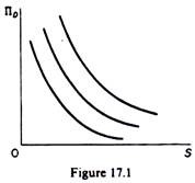
The indifference curves of managers will be drawn on a graph on whose axes we measure staff expenditure (S) and discretionary profit (ΠD). Each indifference curve shows combinations of S and ΠB which give the same satisfaction to the managers. It is assumed that the indifference curves of managers are of the usual shape: they are convex to the origin implying diminishing marginal rate of substitution of staff expenditure and discretionary profit (figure 17.1).
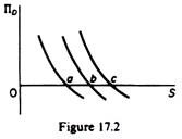
It is further assumed that the indifference curves do not intersect the axes. This assumption restricts the choice of managers to positive levels of both staff expenditures and discretionary profits, implying that the firm will choose values of ΠD and S ‘that will yield positive utility with respect to each component of its utility function’. This means that the model in this version excludes corner solutions, such as points a, b, c, etc., (in figure 17. 2), where ΠD would be zero in the final equilibrium of the firm.
The relationship between S, staff expenditure, and ΠD, discretionary profit, is determined by the profit function
Π= ƒ(X) = f(P, S, s)
since t and Π0 are exogenously given (by the tax laws and the demand for dividends of shareholders).
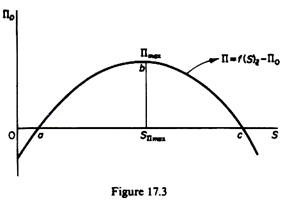
Assuming that output is chosen optimally (according to the marginalistic rule MC — MR) and that the market environment is given (Ɛ), the relationship between Π 0 and S is shown in figure 17.3.
At the initial stages of production and up to the level of output where profits reach their maximum level (point b in figure 17.3) both discretionary profits and staff expenditures increase. However, if production exceeds this level, profits will start declining, but staff expenditures continue to increase. If these expenditures exceed point c, the minimum profit constraint is not satisfied and hence points to the right of c (and to the left of a) are not feasible solutions. It should be clear from the above discussion that the drawn profit curve does not include the minimum profit requirement Π0.
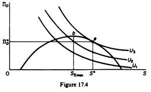
An alternative way of showing the minimum acceptable profit would be to draw the profit function Π = ƒ(S)p,Ɛ and show Π0 as in Baumol’s model, by a straight line parallel to the S-axis. The advantage of subtracting Π0 from each level of actual profit (Π) is that we can reduce the constrained maximisation problem into an unconstrained one. The equilibrium of the firm is determined by the point of tangency of the profit-staff curve with the highest possible managerial indifference curve (point e in figure 17.4).
Given that the indifference curves have a negative slope, it follows that the equilibrium solution will be always on the falling section of the profit-staff curve. This shows the preference of managers for staff expenditure: in Williamson’s model the staff expenditure (S*) will be greater than that of a profit maximiser (SΠmax). Furthermore, Williamson’s model implies higher output, lower price and lower level of profit than the profit- maximisation model. The above predictions will be better understood after the presentation of the general model of managerial discretion.
B. The General Model of Managerial Discretion
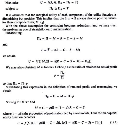
Formally the model may be stated as follows:
ADVERTISEMENTS:
The tax rate t, and the minimum profit requirement Π0 are given exogenously. Hence the utility function depends on three variables output X, staff expenditure S, and the proportion ρ. These are the policy variables of the firm the managers will choose such values for X, S and p so as to maximise U.
In the maximisation procedure we will denote the first partial derivatives of U with respect to S, M and ID by U1 U2 and U3 respectively, that is
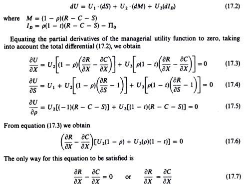
The first-order conditions for a maximum require that the first partial derivatives be equal to zero. (Note that the second-order conditions are satisfied by the assumption of diminishing but positive marginal utilities of the three components of the managerial utility function.) In the maximisation procedure we will use the total differential of the managerial utility function
ADVERTISEMENTS:
given that all the elements in the second expression of the left-hand side of (17.6) are positive by assumption. Thus from the partial derivative of the managerial utility function with respect to x we conclude that in Williamson’s model the firm makes its production decision in the conventional way by equating marginal production cost to marginal revenue.
From equation (17.4), solving for SR/8S, we obtain
Given that by assumption all the elements appearing in the fraction are positive, it follows that
∂R/∂S < 1
ADVERTISEMENTS:
This finding implies that at equilibrium the managerial firm will employ administrative staff beyond the optimal level (that is, beyond the point where the marginal cost of staff is equal to its marginal revenue). Thus there is a tendency for the managerial firm to overspend on staff, to employ more administrative staff than a profit-maximising firm.
From equation (17.5) we obtain
(R- C – S) [-U2 + U3( 1 – t)] = 0
For this equation to be satisfied the second factor must be equal to zero (since (R — C – S) > 0), that is,
-U2 + U3(1 – t) = 0
or
ADVERTISEMENTS:
U2 = (1 – t)U3 (17.9)
This finding shows that in Williamson’s model some amount of profit will be absorbed as emoluments, the amount depending on the tax rate the higher t the smaller U2/U3, the smaller the marginal rate of substitution of emoluments for discretionary investment, and the more will be spent on M and the less on discretionary investment. Given that the marginal utilities have known values.
