Study Notes on the Tax Revenue Function | Econometrics

The below mentioned article provides a study note on the tax revenue function.

The responsiveness of Gross Tax Revenue to the changes in Gross Income is referred to as the Tax Buoyancy. The Tax Buoyancy is also defined as the ratio of proportionate change in gross tax revenue to the proportionate change in Income. The numerical estimate of tax buoyancy is very useful to understand the revenue performance of the economy. Tax Buoyancy can be estimated between two points of time or over a period of time.

Between two points of time, the tax buoyancy [e_Yt..Xt] will be estimated as follows:

Tax Revenue Function Y = f (X) Where

Y = Gross Tax Revenue and

X = National Income.

The rate of change in gross tax revenue per a unit change in National Income will be estimated as follows:

ΔY/ΔX= Y_t– Y_t-1/X_t – X_t-1

This is also known as marginal propensity to gross tax revenue [marginal effect].

In order to calculate the tax buoyancy between two points of time, the following formula will be used:

e_y.x = Y_t – Y_t-1/Y_t-1/X_t – X_t-1/X_t-1

Where

Y_t = Gross tax revenue in ‘t’ year [current year]

Y_t-1 = Gross tax revenue in t-1 year [previous year]

X_t = National Income in ‘t’ year [current year]

X_t-1 = National Income in t-1 year [previous year]

Thus, the ratio of proportionate or percentage change in gross tax revenue to the proportionate or percentage change in National Income is known as Tax Buoyancy.

Tax Buoyancy [responsiveness of Gross Tax Revenue to the changes in Income] will also be estimated as summary statistic over a period of time using OLS method. The tax buoyancy will also be estimated across the states/countries at a point of time. The estimate of Tax Buoyancy can be estimated both from the linear and log-linear regression models.

Linear Tax Revenue Function:

The linear regression model relating to the tax revenue function will be specified as follows:

Y_t = b₀ + b₁X_t + U_t ………………(70)

Where

b₀ = Trend value [estimated value] of tax revenue in the absence of income, known as an intercept. The sign of b₀ will be positive: b₁ = Value of the rate of change in gross tax revenue per a unit change in income, which is known as slope.

The derivative of Y_t with respect to X_t,

[dY_t/dX_t] = b₁, is the rate of change in tax revenue per a unit change in income which will be constant

U_t = the random variable with the usual assumptions. The values of b₀ and b₁ will be estimated by OLS method.

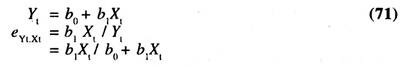
The tax buoyancy [technically speaking it is a responsiveness of gross tax revenue to the changes in gross income] will be estimated from the linear regression model as follows:

Thus, b₁ is a component of tax buoyancy. Tax buoyancy varies from point to point changes in X_t and Y_t. The tax buoyancy is directly related to the increase in income and inversely related to increase in tax revenue. In empirical Studies, the numerical value of tax buoyancy is evaluated at the mean values of tax revenue and national income.

e_Yt.Xt = ∂Y_t/∂X_t . mean of X_t/mean of Y_t = b₁. mean of X_t/mean of Y_t

Therefore, the estimate is called as an average tax buoyancy. Further it should be noted that the probable value of the tax buoyancy can be ascertained on the basis of the sign of the intercept, b₀, in the simple linear regression model.

This can be understood from the following equation:

If the sign of b₀ is positive then the average tax buoyancy will be less than unity; if the sign of b₀ is negative then the average tax buoyancy will be more than unity; if the sign of b₀ is zero, then the average tax buoyancy will be unity. Thus, on the basis of the sign of the intercept, the size of the tax buoyancy will be ascertained from a simple linear regression model.

In time series data, the tax buoyancy will also be estimated by taking the ratio of the growth rate of tax revenue to the growth rate of national income.

In a linear regression model, the linear growth rate of tax revenue will be estimated as follows:

Y_t = b₀ + b₁t………………. (72)

Where

Y_t = Gross tax revenue [Dependent variable in a simple linear tax revenue function]

t = Time in years.

b₁ = Rate of change in tax revenue per year

b₀ = Trend value of tax. revenue, when t = 0

The Linear Growth Rate of tax revenue [LGR_y] from the above equation will be estimated as follows:

LGR_y = Marginal tax revenue function/Total tax revenue function * 100

= dY / dt / Y.1 = [dY / dt. 1 / Y] .100

= b₁/Y.100.

In empirical studies the value of Y is the average of Y series.

Similarly the linear growth rate of national income [LGR_X] will be estimated as follows:

X_t = b₀ + b₁t ……………(73)

Where

X_t = National Income [Independent variable in the simple linear tax revenue function]

b₁ = Rate of change in National Income per year.

The linear growth rate of national income [LGR_x] will be calculated as follows:

LGR_X = Marginal income Function/Total income Function

= dX₁ /dt / X= .100 = [dX₁ / dt . 1 / X_t] .100

The ratio of the linear growth rate of tax revenue to the linear growth rate of income is the estimate of tax buoyancy.

Thus, the growth rates of gross tax revenue and income will be used to know the degree of tax buoyancy. If the estimate of tax buoyancy is more than unity (1) then the growth rate of tax revenue will be relatively higher than the growth rate of income. (2) If it is less than unity, then the growth rate of tax revenue will be relatively smaller than the growth rate of income and (3) If it is unity, then the growth rate of tax revenue will be equal to the growth rate of income.

The estimation of tax buoyancy from the linear regression model is based on the assumption of linear relationship [constant rate of change between tax revenue and income] between tax revenue and income. If the linear relationship does not exist between them, the other forms of regression equations such as power function [log linear regression model] will be attempted for estimating the tax buoyancy.

Log Linear Tax Revenue Function:

In empirical studies, the tax buoyancy will also be estimated using the following power function;

Y = b₀X₁^b1

For the purpose of estimation by OLS method, the equation will be transformed into a log linear model

log Y = logb₀ + b₁ logX……………. (74)

The derivative of log Y with respect to log X,

d log Y / d log X, is, the constant tax buoyancy

d log Y / d log X = dY / Y / dX / X = dY / Y.X / dX

= dY / dX.X / Y = b₁

The tax buoyancy in the above equation will also be estimated by taking the ratio of the instantaneous growth rate of tax revenue to an instantaneous growth rate of national income.

This can be shown as follows:

log Y = log b₀ + b₁t ………………..(75)

The derivative of log Y with respect to t

= d log X / dt = dX / X/ dt / 1 = dX / X.1/ dt =

1 / Y dY / dt = b₁ will be an instantaneous growth rate of tax revenue.

log X = log b₀+ b₁t ………………(76)

The derivative of log X with respect to t

= d logX/ dt = dX /X / dt / 1 = dX / X.1/ dt =

1 / X dX /dt = b₁ will be an instantaneous growth rate of National Income.

The ratio of growth rate of gross tax revenue to that of national income, dY / dt 1 / Y / dX / dt. 1 / X

= dY / dtY. dtX / dX

= dY / dX. X / Y is referred to as an estimate of tax buoyancy. If the degree of tax buoyancy is more than unity, then the instantaneous growth rate of tax revenue will be relatively higher than that of instantaneous growth rate of national income. If the degree of tax buoyancy is less than unity, then the instantaneous growth rate of tax revenue will be relatively smaller than the instantaneous growth rate of national income.

If the degree of tax buoyancy is unity, then the instantaneous growth rate of tax revenue will be equal to the growth rate of national income. Thus, the log-linear form of regression equation of tax revenue on income will be helpful in ascertaining the size of the instantaneous growth rates of tax revenue and national income.

It should be noted that the estimate of tax buoyancy through the log-linear equation will be constant. In the empirical studies, log linear form of regression equation is being widely used to estimate the degree of tax buoyancy on the grounds that the regression coefficient of log X [income] gives directly the size of tax buoyancy. So far the discussion is confined to the short-run tax buoyancy.

Short Run and Long Run Tax Revenue Functions:

The long-run tax buoyancy will also be estimated using Nerlovian Partial Adjustment Model [mechanism] as follows:

The long-run linear tax revenue function can be specified as follows:

Y_t* = b₀ + b₁X_t …………………(77)

Where

Y_t* = Desired/ Equilibrium/Long run/ Optimal level of tax revenue collections. As this variable is not observable, the following partial adjustment mechanism will be taken into consideration to estimate the short-run tax revenue function, which is basis for estimating long-run tax revenue function.

[Y_t – Y_t-1] = δ [Y_t*-Y_t-1] ……………(78)

Where

(Y_t – Y_t-1] = Actual change in the collection of tax revenue

[Y_t* – Y_t-1] = Desired change in the collection of tax revenue

δ = coefficient of Partial Adjustment whose value will be more than zero and less than or equal to 1. If it is less than one, then the actual change in tax revenue will be smaller than the desired change in tax revenue. If it is one, then the actual change will be equal to desired change. If it is zero, then there will be no change between Y_t and Y_t-1. That is [Y_t – Y_t-1]= 0.

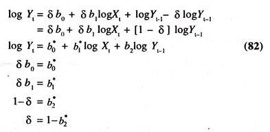
If the above equation is substituted in the long-run linear tax revenue function, then we obtain the following equation:

 

 

 

 

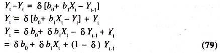
Y_t = b₀* + b₁*X_t + b₂Y_t-1 : This is known as the short-run tax revenue function. The tax revenue in current year depends on income in current year and tax revenue in previous year

Where

The short run tax buoyancy will be estimated at the mean values of Y_t and X_t as follows:

= b₁* mean of X_t/mean of Y_t

The long-run tax buoyancy will be estimated by deflating the short-run tax buoyancy with δ.

LRE = b₁* mean of X_t/mean of Y_t* 1/δ

The long-run tax revenue function will be estimated by deflating the short-run tax revenue function with δ and omitting Y_t-1 .

This function is based on the assumption of linear relationship between tax revenue and income. If the linear relation does not exist, then the following form of non-linear relationship will be attempted.

For the purpose of making estimates, this function is transformed into the following form:

log Y* = log b₀+ b₁ log X_t…………… (80)

Since Y* is not observable, this function [long run tax revenue function] will be estimated by the short-run revenue function generated through the partial adjustment model [mechanism]. The partial adjustment model is

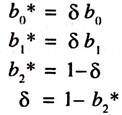
For the purpose of estimation, the above model is transformed into the log linear form as follows:

By substituting the above equation in the partial adjustment mechanism we get the following short ran tax revenue function.

Thus, the lagged dependent variable, logY_t-1, is entered the equation as one of the independent variables. The derivative of log Y_t with respect to log X_t is short-run estimate of tax buoyancy

The long-run tax buoyancy will be estimated by deflating the short-run tax buoyancy by the coefficient of partial adjustment [δ] as follows:

Thus, the estimate of long-run tax buoyancy will be calculated by partial adjustment mechanism. In empirical studies, the estimates of tax buoyancy for different types of taxes are estimated using time series data by the OLS method. Since, the estimates are based on time series data the econometric problem of auto-correlation needs to be reduced by using the first difference method.

The process of differencing the variables will continue till the Durbin-Watson statistic turns out to be two. Apart from income, the impact of tax rate will also be examined on tax revenue. Sometimes, to capture the impact of time on revenue, the time variable will also be included in the tax revenue function.

In such cases, the functional relationship between tax revenue and national income, tax rate and time variable will be specified as follows:

Where

Y = Tax Revenue

X_1t = National Income

X_2t = Tax Rate

X_3t = Time Variable in Years

If the above function is specified in a multiple linear regression form, we get the following econometric model.

Y= b₀ + b₁X₁ + b₂X₂ + b₃ X₃ + U…………….. (83)

Where

b₁ = ∂Y/∂X₁, is the rate of change in Y per unit change in X₁

b₂ = ∂Y/∂ X₂, is the rate of change in Y per unit change in X₂

b₃ = ∂ Y/∂ X₃, is the rate of change in Y per unit change [one year] in X₃

These are constants and concerned with marginal effects. The estimate of the tax buoyancy from the above function will be variable, if they are evaluated at different values of Y and X₁.

The responsiveness of Y to the changes in X , all else equal, can be understood from b₁.Y/X₁ Similarly, the responsiveness of Y to the changes in the tax rates can be understood from b₂ Y/X₂.

If the linear relationship between Y and X₁, X₂ and X₃ does not exist then the other form of equation such as log linear model will be attempted

log Y = logb₀ + b₁logX₁ + b₂log X₂+ b₃ X₃ …………………(84)

The partial derivative of log Y with respect to logX₁, b₁, is the constant tax buoyancy, while the partial derivative of log Y with respect to X₂, b₂, is the degree of responsiveness of tax revenue to the changes in tax rates [This helps to understand whether the laffer curve (An inverted U shape relationship between the revenue from direct taxes and tax rates) is operating in the economy or not (See Table-8.11 for the regression results on empirical validity of laffer curve). The partial derivative of log Y with respect to X₃, b₃ is the instantaneous growth rate of tax revenue, i.e.

Thus, the tax buoyancy will be estimated from the linear and log-linear forms of simple and multiple regression equations by using OLS method. This method will be followed on the grounds that there is one way causation between the tax revenue and each of the independent variables.

In other words, the co-variance between income and random variable, and covariance between tax rate and random variable must be zero. If this assumption is not fulfilled, then the estimates will be biased. To reduce this bias either the two stage least squares method [TSLSM] or [ILSM] indirect least squares method will be used.

Tax Revenue Function-Estimates of Economic Relationships:

The data given in Table 8.1 are used to explain the tax revenue function.

Visual Plot:

The Tax Revenue and Income series move together in the same direction [Figure – 8[A]]

The regression results of the linear tax revenue function [Table 8.2] based on the data given in table 8.1 show that the regression coefficient of income is significantly positive. This is known as marginal propensity to gross tax.

The value of tax buoyancy estimated at the mean values of Y and X [0.0865*(720419.2/67392.15)] is 0.925 showing that if the income is increased by one per cent, the tax revenue is likely to increase by 0.925 per cent per annum, all else equal. Since the value of tax buoyancy is less than unity, the buoyancy of tax is relatively inelastic.

The data given in table 8.3 are used to fit the log linear tax revenue function for explaining the estimate of constant tax buoyancy.

The regression results of log linear tax revenue function [Table 8.4] show that the regression coefficient of log income [tax buoyancy] is 0.97. According to the value, it can be inferred that a one percent increase in national income leads to increase the tax revenue by 0.97 percent per annum. In the log linear tax revenue function also, the size of the tax buoyancy is found to be less than unity showing that the tax buoyancy is relatively inelastic.

The regression results presented in table 8.6 based on the data points given in Table 8.5 explain the presence of shift / structural change / break in the magnitude of tax buoyancy after having ensured that the time series variables are stationary. As the consistent statistical deduction from macro time series depends on the assumption, of stationarity, it is sensible to determine whether time series variables, log (Y_t) and log (X_t), are individually stationary or non-stationary.

If they are non-stationary, then the concern is to what degree/order they are non-stationary. Therefore the order of integration of each variable is examined by the Augmented Dickey-Fuller [ADF] test in levels on log (Y_t) and log (X_t) [Equation-85 and Equation-86] before the advent of the estimation of the coefficients of tax buoyancy during pre tax reform period [ β₁] and differential tax buoyancy during post tax reform period [β₃] [Equation-87] by ordinary least squares method.

If the calculated ADF statistic is more than its critical value then the variable [log (Y_t) or log(X_t)] is said to be stationary or integrated to the order zero in log level i.e., log(Y_t)~I(0) and log(X_t) ~ I(0).

If the calculated ADF statistic is less than its critical value then the time series variable [log(Y_t) and log(X_t)] is said to be non-stationary in log levels Then the ADF test will be performed on the first difference of log (Y_t) and log (X_t) [i.e., ADF unit root test on Δ log (Y_t) = log Y_t – log Y_t-1 and Δ log(X_t)= log X_t – log X_t-1].

If log Y and log X are found to be stationary in first difference, then they are integrated to the order one i.e., log (Y) ~ I(1) and log (X) ~ I(1). Indeed the ADF unit root test in first difference is not performed here as the ADF statistic in level is found to be significantly negative. The results of the ADF tests with intercept and trend are presented in table 8.7.

The ADF unit root test [in level] on log Y [equation 85] and log X [equation 86] is based on the following regression

 

 

 

 

 

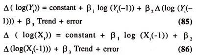
Where Δ log is the first difference [operator] of the log of the variable [log (Y_t) or log(X_t)].The null hypothesis that the time series variable [log(y_t) and log(X_t) ] has a unit root [ i.e., it is non stationary ] is rejected as p , the regression coefficient of log (y_t(-1) in equation (85) and the regression coefficient of log (X_t(-1)) in equation (86) is significantly negative.

The results illustrate that the non stationarity/unit root can be rejected for the log levels of the variable Y at one percent level and X at ten percent level of the significance as the calculated ADF statistic is more than MacKinnon critical value. Therefore the time series variables [log (Y) and log(X) ] in log levels are stationary ie., log(Y_t) ~ I(0) and log (X_t) ~ I (0). The OLS method can be applied to estimate the degree of tax buoyancy.

Differential Tax Buoyancy:

The degree of differential central tax buoyancy during post tax reform period is scanned by fitting the following form of regression model [Equation -87] with an interaction variable[D*logX_t]

log Y_t = log β₀ + β₁ logX_t + β₂ D + β₃ (D * log X_t) + error ….(87)

Where

Y_t= Central Tax Revenue [Rs crore]

X_t = Gross Domestic Product [gdp]at market prices (Income) [Rs crore]

β₀= Intercept during pre tax reform period [D = 0]

β₂ = Differential intercept during post tax reform period [D = 1]

β₁ =Magnitude of tax buoyancy during pre tax reform period (D = 0); β₁> 0

β₃ = Magnitude of differential tax buoyancy during post tax reform period (D = 1); β₃ more than or less than zero evincing the difference between the magnitude of tax buoyancy during post tax reform period and magnitude of tax buoyancy during pre tax reform period

(β₁ ± β₃) = Magnitude of tax buoyancy during post tax reform period (D = 1)

If the regression coefficient of dummy variable [D], β₂ is significantly positive then the average central tax revenues would go up during post tax reform period [D =1]; If it is significantly negative, then the average tax revenues would go down. Β₁ = regression coefficient of tax buoyancy [β₁ > 0] during pre-tax reform period [1951 to 1992] when D = 0, β₃ = differential coefficient of tax buoyancy [ β₃ more than or less than 0] that allows a shift [an upward/a downward] in the tax buoyancy during post tax reform period [1993 to 2000 ] when D =1.

As the interaction variable [D*log X_t] enters the equation in dichotomous form [i.e.,D = 0 in pre tax reform period and D = 1 in post tax reform period] the derivative of logY_t with respect to [D*log X_t] does not exist. Instead, the coefficient of [D*logX_t] subject to statistical significance, measures the discontinuous effect of the presence of the attribute [D = 1] represented by an interaction variable on the tax revenue.

The variable [D*log X_t], which is an interaction variable, is introduced in model [equation-87] to capture the interaction effect of post tax reforms and income on the revenue from major taxes.

The interaction variable takes a value equal to log X_t during post tax reform period [when D = 1] and 0 during pre tax reform period [when D = 0] ; If [β₁* ± β₃*] more than or less than β₁* then there will be an upward or a downward shift in the degree of tax buoyancy during post tax reform period; If [β₁* + β₃**] = β₁*, then there will be a homogeneity in the magnitude of tax buoyancy i.e., magnitude of tax buoyancy remains the same in pre and post tax reform periods implying the absence of differential tax buoyancy. Where * and ** denote statistically significant and insignificant respectively.

Degree of Differential Tax Buoyancy:

As the time series log variables are found to be stationary in their level, log(Y_t) ~ I(0) and log (X_t) ~ I (0), the degree of tax buoyancy during pre tax reform period and differential tax buoyancy during post tax reform period can be estimated by fitting the double log regression model [Equation-87] by OLS method. The results based on the data given in table 8.6 are presented in table 8.8.

The numerical values of the regression results illustrate that the estimate of constant tax buoyancy is more than unity and significant during pre tax reform period revealing that if income increases by one percent on the average the gross tax revenue goes up by 1.24 percent, all else equal.

The regression coefficient of interaction variable, which is differential tax buoyancy, is significantly negative showing that the tax buoyancy is less than unity during post tax reform period. The estimate of the tax buoyancy, which is just above the unity, has come down by 0.362 points during post tax reform period.

The size and sign of the differential tax buoyancy coefficient show the absence of an upward shift in the degree of tax buoyancy during post tax reform period. Thus the estimates of tax buoyancy in pre and post tax reform periods are different. This analysis is surmised in table 8.9.

 

Validity of Laffer Curve:

The relationship between tax rate [X₁] and tax revenue[Y] will be studied by fitting the following form of quadratic equation without intercept

Income Tax Revenue [Y] = b₁ (Tax Rate) – b₂ (Tax Rate)²

The above equation is mathematically derived for empirical estimation of the laffer curve [An inverted U shape relationship between income tax revenue [Y] and tax rate [X]] as follows.

Tax revenue [Y] is equal to the tax rate [X₁] times the base

[X₂] i.e.,y = X₁*X₂ …………….(88)

The inverse relationship, which is assumed to be linear, between X₁ and X₂ will be expressed as follows

X₂ = b₁– b₂ X₁ …………………..(89)

Substituting the equation [89] into equation [88] the following equation will be obtained

Y = X₁ [b₁ – b₂X₁]

= b₁X₁ – b₂ X₁² ………………(90)

Thus the empirical estimation of the laffer curve is based on equation [90]. If the intercept [to take the value (non zero) of Y, which is trend value in the absence of X₁ on vertical axis] is included in the equation [90], then the form of the equation [Quadratic equation] will be as follows:

Y = b_{0 +} b₁X₁ – b₂ X₁² ……………(91)

The derivative of Y with respect to X₁

dY / dX₁ = b₁ – 2 b₂X₁ [The marginal tax revenue goes on declining with the increase in tax rate]

By setting the derivative to zero, the value of the marginal tax rate can be worked out to know the maximum tax revenue.

 

 

 

 

The first derivative [necessary condition] must be zero and second derivative[sufficient condition] must be < 0

The second derivative= d²Y/dX₁ ² = – 2b₂ < 0

The data given in Table 8.10 on revenue from income tax [Y] tax rates [X₁] and its square [X²] are used to explain the robustness of the income tax laffer curve

The regression results of the quadratic regression model [Table 8.11] without intercept [curve starts from the origin] show that the regression coefficient of maximum marginal tax rate and its square are significant.

The sign of X is positive and that of X¹ is negative confirming that the income tax laffer curve is operating. The concern here is that only 18 percent of the total variation in Y is explained by both X and X² together. Therefore due attention is required to explain the results of the empirical studies.