Differential Coefficients in Error Correction Model [Degree of Differentia] Disequilibrium and Correction in Short Run]
Once the cointegration [long run equilibrium] between two variables is established, the impact of qualitative variable on first differenced dependent variable [ΔYt or ΔXt] can be examined in error correction model [ECM] to mainly know the degree of differential disequilibrium between short run and long run values [which can be eliminated] by including dummy and interaction variables 1] dummy variable times error correction term in lagged period ( D*ECt-1) and 2] dummy variable times Δ log Xt(D*Δlog Xt) or dummy variable times Δ log Yt (D*Δ log Yt)
ECM in case of Y on X:
Δ log Yt = b0+ b1 D + b2 Δ log Xt + b3(D*Δ log Xt) + b4 ECt-1 + b5 ( D*ECt-1) + error……………… (129)
ADVERTISEMENTS:
Where
Δ log Yt and Δ log Xt are first differenced variables [Stationary variables with the same order of integration]
D = Dummy variable that takes value 0 in the absence of attribute [for example Pre economic reform period in India] and 1 in the presence of attribute [ Post economic reform period in India ]
D*Δ log Xt= Interaction variable that takes value 0 in the absence of attribute i.e. D*Δ log Xt = 0 and 1 in the presence of attribute i.e. D*Δ log Xt= Δ log Xt
ADVERTISEMENTS:
D*ECt-1 = Interaction variable that takes value 0 during pre economic reform period [in the absence of attribute ] i.e. D*ECt-1 = 0 and 1 during post economic reform period [in the presence of attribute] i.e. D*ECt-1 = ECt-1
b0 =Intercept during pre economic reform period [D=0]
b1 = Differential intercept during post economic reform period [D=1]
The sum of b0+b1 is the size of intercept during post economic reform period [D=1]
ADVERTISEMENTS:
b2= coefficient of Δ log X, [constant elasticity] during pre economic reform period [D=0]
b3= Differential coefficient of Δ log Xt [differential constant elasticity ]during post economic reform period [D=1]
The sum of b2 and b3 is the size of coefficient of Δ log Xt [size of constant elasticity] during post economic reform period. [D=1]
b4= Coefficient of error correction term [constant elasticity] in t-1 period in the absence of attribute [D=0] and expected sign will be negative
b5= Differential coefficient of error correction term [differential constant elasticity] in t-1 in the presence of attribute [D=1], If the sign of the differential coefficient is significantly negative then the degree of disequilibrium in t-1 period will quickly be eliminated in t period.
The sum of – b4 and – b5 will be the size of coefficient of error correction term in t-1 period in the presence of attribute [D=1]
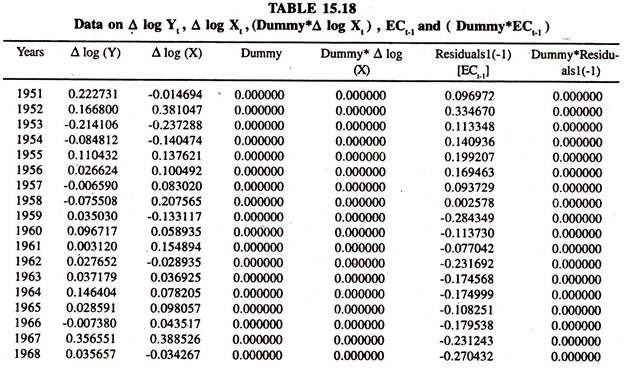
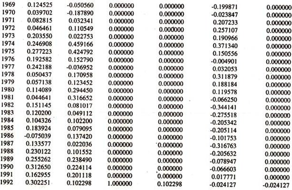
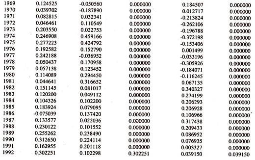
The data given in table 15.18 are considered to estimate the ECM.
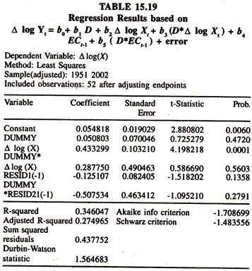
The regression results of the ECM are given in table 15.19
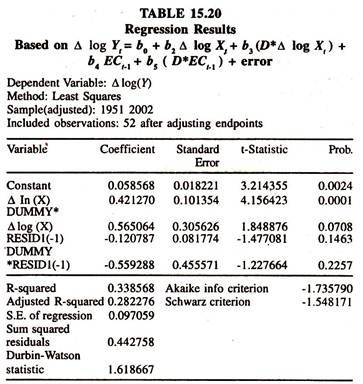
Since the coefficient of dummy variable [differential intercept] is found to be statistically insignificant, the ECM is fitted to the data by deleting this variable [D] from the model. The results of the same are given in table 15.20.
ADVERTISEMENTS:
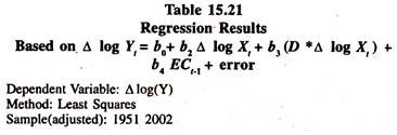
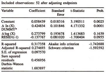
The results of the model show that the differential coefficient of the error correction term is found to be statistically insignificant. Therefore deleting the interaction variable as well the ECM is fitted to the data. The results of the same are given in table 15.21.
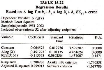
The results of the ECM show that the differential coefficient of an interaction variable [DUMMY* A log Xt ] is also found to be statistically insignificant. Therefore deleting an interaction variable as well the ECM is fitted to the data.The results of the same are given in table 15.22.
ADVERTISEMENTS:
The results of the ECM show that the coefficient of error correction term is negative but not significant showing short run equilibrium. Thus the step wise regression results [by deleting the insignificant variables] show the presence of short run equilibrium both in pre and post economic reform periods.
ECM in case of X on Y:
ADVERTISEMENTS:
Δ log Xt and Δ log Yt are first differenced variables [Stationary variables with the same order of integration]
D = Dummy variable that takes value 0 in the absence of attribute [for example Pre economic reform period in India] and 1 in the presence of attribute [Post economic reform period in India]
D* Δ log Yt= Interaction variable that takes value 0 in the absence of attribute i.e. D*Δ log Yt = 0 and 1 in the presence of attribute i.e. D*Δ log Yt= Δ log Yt
D*ECt-1 = Interaction variable that takes value 0 during pre economic reform period [in the absence of attribute ] i.e. D*ECt-1 = 0 and 1 during post economic reform period [in the presence of attribute] i.e. D*ECt-1= ECt-1
b0= Intercept during pre economic reform period [D = 0]
ADVERTISEMENTS:
b1= Differential intercept during post economic reform period [D = 1]
The sum of b0+b1 is the size of intercept during post economic reform period [D = 1]
b2= coefficient of Δ log Yt during pre economic reform period [D = 0]
b3 = Differential coefficient of Δ log Yt during post economic reform period [D =1]
The sum of b2 and b3 is the size of coefficient of Δ log Yt during post economic reform period [D = 1]
b4 = Coefficient of error correction term in t-1 period in the absence of attribute [D = 0] and expected sign will be negative
ADVERTISEMENTS:
b5 = Differential coefficient of error correction term in t-1 in the presence of attribute [D = 1]. If the sign of the differential coefficient is significantly negative then the degree of disequilibrium in t-1 period will quickly be eliminated in t period.
The sum of – b1 and – b2 will be the size of coefficient of error correction term in t-1 period in the presence of attribute [D = 1]
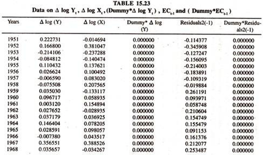
The data given in table 15.23 are used to estimate the ECM.
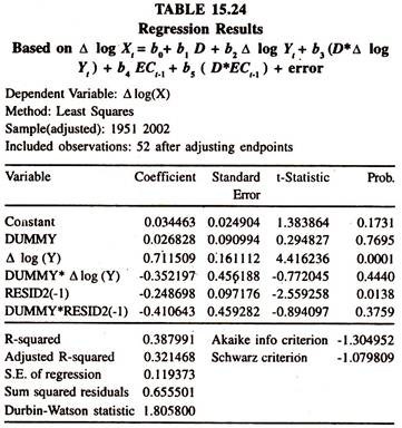
The results of the ECM specified in the appendix are given table 15.24.
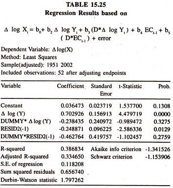
Since the coefficient of dummy variable is found to be statistically insignificant, the ECM is fitted by deleting this variable [D] from the model. The results of the ECM are given in table 15.25
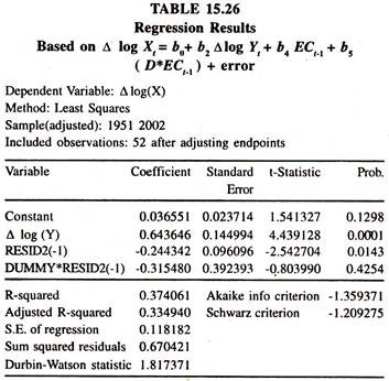
The regression results of ECM show that the coefficient of interaction variable [D* Δ log Y ] is insignificant. Therefore the ECM is fitted by deleting the interaction variable. The results are given in table 15.26
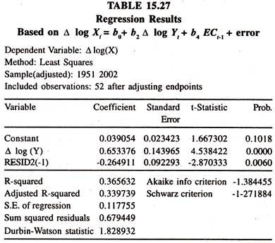
The regression results of the ECM show that the coefficient of interaction variable [D*ECt-1] is as well found to be insignificant. Therefore the ECM is fitted by deleting the interaction variable. The results are given in table 15.27.
The results of the ECM show that the coefficient of error correction term is statistically found to be significant evincing short run disequilibrium between short run and long run values. Further the coefficient shows that the degree of error correction between short run and long run by changes in imports every year is twenty six percent both in pre and post economic reform periods.
