Study Notes on the Supply Response Function | Econometrics

The below mentioned article provides a study note on the supply response function.

Linear Supply Response Function:

In the field of agriculture, a large number of empirical studies are carried out using time series data to know the responsiveness of the area [acreage] under the crop [Supply] to the changes in the prices in lagged year. This is known as the supply response/acreage response function.

It is quite common that the cultivators take the decisions of allocating the area under the crop by considering the previous year prices. If prices in the previous year were higher, then the cultivators will be induced to allocate more area under the crop as compared to the area cultivated in the previous year. Thus the decision of allocating the area under a particular crop depends mainly on the previous year prices.

It is common that there will be a desired level of area that will be brought under the cultivation of a crop. The cultivators attain the desired level of area gradually, not instantly, due to various factors. The desired level of area to be brought under cultivation will be the function of the prices of the crop in last year.

This is known as long-run supply response function [Acreage Response Function]. The desired level of area under the crop is unobservable.

In order to estimate the long-run supply response function, the Nerlovian’s Partial Adjustment Mechanism will be followed:

 

 

Where

A_t = Area under the crop [food crop or non food crop] in the current year.

A_t-1 = Area under the crop in the lag year.

δ = Coefficient of adjustment [speed of adjustment], whose value will generally be more than zero and less than unity.

A_t* = Desired equilibrium level of the area under crop [which is not observable]

[A_t –A_t-1 ] = Actual change in the area

[A_t*—A_t-1] = Desired change in the area

The long-run linear supply response function will be specified as follows:

 

 

Where

A_t* = As defined above

P_t-1 = Average price of the crop in lag year

U = Random variable

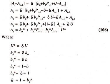
In order to estimate the long run supply [Acreage] response function, the equation (105) is substituted in equation (104) to obtain the short run supply response function.

 

 

 

 

 

 

 

 

 

 

 

b₁* is the rate of change in area under cultivation per a unit change in the lag year prices.

i.e., ∂A_t/∂P_t-1=b₁*

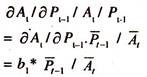
The responsiveness the area under cultivation with respect to the changes in lag year prices will be evaluated at the mean values [P̅_t-1 and A̅_t] as follows:

 

 

 

This is known as the short run [Short run elasticity reflects a time period that is not long enough for Farmers / Producers to adjust completely the desired area to the changes in prices] average price elasticity of acreage as it will be estimated at the mean values.

If the value is more than unity, then the short run price elasticity will be relatively more elastic. If it is less than unity, then the price elasticity will be relatively inelastic. If it is unity, then there will be unitary price elasticity.

The long-run Price elasticity [Refers to the situation where the Farmers/Producers have more time to adjust the desired area to the changes in prices] will be evaluated as follows:

Short run price elasticity/coefficient of partial adjustment

 

 

 

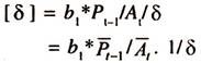
The long-run price elasticity will be relatively higher than the short-run price elasticity as the value of coefficient of adjustment [δ] will generally be less than unity. The long-run price elasticity shows the cumulative effect of the changes in prices on the area under cultivation. The coefficient of adjustment (δ), shows the speed of adjustment between the desired change in acreage [A_t* – A_t-1] and actual change in acreage [A_t – A_t-1 ].

If its value is unity, then there will be an instantaneous adjustment in that year between the desired change in acreage and actual change in acreage. If it is less than unity, then the actual change in acreage will be lower than desired change in acreage. Thus, the value of coefficient of adjustment (δ) shows the speed of adjustment between the actual change and the desired change in the area under cultivation.

The above equation of supply [acreage] response function would be appropriate, if there exists a linear relationship between the area under cultivation in current year and price in lag year. If it is not linear, then the other forms of supply response functions have to be attempted.

Log Linear Supply Response Function:

In the empirical studies the log-linear form of supply response function is being fitted to the time-series data. The regression coefficients of the price in a lagged year gives directly the value of the short run elasticity of the acreage under the crop with respect to changes in price in that lag year.

The specification of log-linear supply response function for a crop [food or commercial] will be as follows:

 

This is known as the long-run supply response function. Since the desired level of area [A_t*] is not observable, the following partial adjustment mechanism will be adopted to estimate the function:

 

 

Substituting the equation (107) in equation (109) we get the following short run supply response function:

 

 

 

 

 

 

 

 

 

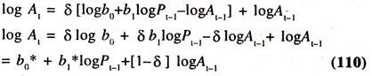
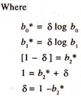
b₁* is the constant short run elasticity [SRE] of the area under the crop with respect to the changes in lagged prices.

b₁* = ∂ logA_t/∂ logP_t-1

The long-run elasticity of acreage with respect to lagged prices will be estimated as follows:

SRE/δ = ∂ logA_t/∂ logP_t-1/δ

= b₁*/δ

The numerical value of the long run price elasticity of acreage would generally be higher than the short run price elasticity as the Coefficient of Partial adjustment would be less than unity.

In empirical studies on supply response function, apart from the prices of the crop in the lagged year, the other variables such as lagged yield, price risk (the coefficient of variation [ratio of standard deviation to the mean of the price variable] based on the preceding three or five years) and yield risk (the coefficient of variation [ratio of standard deviation to the mean of the yield variable variable] based on the preceding three or five years) the average rainfall etc., may also be taken into consideration.

With the advent of software packages on Econometrics, the short-run and long-run supply response functions will easily be estimated. It should however be noted that in time series data, the independent variables move either in the same direction or opposite direction creating a problem of multi-collinearity between the independent variables in the supply response function.

The presence of multi-collinearity between the independent variables breaks the precision of the estimates of elasticities. This problem can to some extent be rectified either by increasing the sample size or deleting unimportant independent variables from the supply response function.

So far as the supply response function in agricultural sector is concerned, a large number of empirical studies are carried out by considering the important variables for different crops in India using Partial Adjustment mechanism. Apart from the above variables, the variables such as the area under irrigation, the prices of other crops etc., may also be considered in the function.

Only important variables which are statistically significant have to be retained in the supply response function for the analysis. The degree of multi-collinearity will be traced out by the correlation matrix.

The high degree of correlation between the independent variables indicates the presence of multicolinearity. Since time series data will be used in supply response function other important problems that will be faced is the auto-correlation. This problem can to some extent be reduced by taking the variables in first difference form.

Supply Response Function-Estimates of Short Run and Long Run Price Elasticities:

The following data [Table 12.1] on area under paddy crop in current year and prices in lagged year are considered for estimating supply response function.

The regression results of the linear acreage [supply] response function [Table 12:2] show that the regression coefficient of the lagged price is significantly positive. The short run price elasticity is 0.3290 [estimated at the mean values of A_t and P_t-1: 0.593614(134.2/242.1) showing that a one percent increase in the lagged price of the Paddy crop induces the farmers to allocate the area under the Paddy crop by 0.329 percent in current year.

The value of coefficient of adjustment [1 – regression coefficient of lagged area = 1- 0.56 = 0.44] explains that the discrepancy [disequilibrium] between actual change and desired change in the area can be eliminated to the extent of 0.44 units every year.

The long run price elasticity [short run price elasticity/coefficient of adjustment: 0.329050/0.44 = 0.7478] explains that the cumulative effect of changes in the price on the current year’s acreage is such that if the lagged price is increased by one percent then the area under the crop in current year will be increased by 0.748 percent per year.

The value of coefficient of partial adjustment is less than unity showing the difference between actual change and desired change in the area. If the linear supply response model is not appropriate to time series data, then other form such as log-linear supply response function needs to be considered.

The data [transformed into logarithms] given in table 12.3 are considered to estimate the log linear supply response function.

The regression results [based on the data furnished in Table 12.3] of the log linear supply response function [Table 12.4] show that the regression coefficients of lagged prices and lagged area are the constant short run elasticities.

The regression coefficient of the lagged prices is found to be significantly positive. This is known as the short run price elasticity showing that a one percent increase in the lagged price would increase the area under the crop in current year by 0.32 percent per annum, all else equal.

The coefficient of partial adjustment is 0.462 [1 – 0.538] showing that the discrepancy (disequilibrium) between the desired change and actual change in the area under the crop can be eliminated by 0.46 percent every year.

The long run price elasticity [short run price elasticity/coefficient of partial adjustment [0.321855/0.462 = 0.696656] is 0.70 showing that the cumulative effect of the changes in the prices of the crop over a period of time on the acreage is such that if the price of the paddy crop is increased by one percent in the lagged year then the area under the crop will be increased by 0.70 percent in current year. It should be noted that the long run price elasticity is relatively higher than the short run price elasticity.