Long Run Equilibrium Relationship | Econometrics

In this article we will discuss about the long run equilibrium relationship.

Stationarity of Time Series Data [Augmented Dicky Fuller [ADF] Test]:

Statistical interference from macro economic time series is generally based on the assumption of stationarity of the series, which more often found to be violated in many macro economic time series. If time series data are non stationary then the regression results based on the ordinary least squares [OLS] method will be spurious. Therefore there is a need to test whether the time series variable is stationary or not.

In other words the determination of order of integration of each time series variable is required. This objective will be attained by unit root testing of the time series. The unit root test provides the information about the stationarity of the time series variables. If the time series variable is not stationary, then the series contain unit root.

The presence of unit root in the time series data generates unreliable results regarding the hypothesis testing. Before carrying out hypothesis testing, the non stationary time series data need to be differenced until stationarity has emerged.

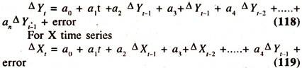
One way of testing for the presence of unit root and for determining the order of integration of each time series variable is to deploy the Augmented Dicky Fuller [ADF] test This test involves the estimation of the following forms of regression equations with intercept and trend

For Y time series:

 

 

 

 

Where

Y_t or X_t = Macro time series economic variable in t period

t = time

Δ = First difference operator

Additional terms [length of the lags] in the first differences [based on Akaike Information Criterion (AIC) and Schwarz Information Criterion (SIC)] to whiten the noise process [Determination of optimal length of the lag will be based on the minimum value of AIC and SIC]. In other words extra lags [t-1, t-2, t-3…………… t-n] will be added until the autocorrelation disappears.

If a₂ [ADF test statistic] is significantly negative and higher than the MacKinnan critical value then the null hypothesis that the Y or X series [any time series macro variable] has unit root [the series is integrated order 1 i.e. Y ~ I(1) or X ~ I(1)] can be rejected. Thus the order of integration of each time series variable will be determined by ADF test statistic.

Cointegrating Regression:

If the time series variables under consideration, Y and X, are the same order of integration [ Y and X ~ I (1)] though they are individually non stationary [The variables individually are not mean reverting], the estimation of regression equation of Y on X or X on Y in level form [or static form] by OLS method is referred to as cointegration regression as shown below

Y_t = intercept + b₁ X_t + error……………. (120)

X_t = intercept + b₁ Y_t + error……………. (121)

Where

b₁ = long run regression coefficient

In order to examine whether there is long run equilibrium relationship between Y and X, [whether they move together in the long run] the stationarity of the residuals/errors [equilibrium error term:U] obtained from the cointegration regression of Y on X or X on Y [equations 120 and 121] has to be tested using ADF test with trend and intercept as shown below:

Residuals /errors [from cointegration regression of Y on X]

Ut = Y_t – [intercept + b₁ X_t ] ……………(122)

Residuals /errors [from cointegration regression of X on Y]

Ut = X_t – [intercept + b₁ Y_t ] ………………..(123)

ΔU_t = intercept + b₁t +b₂ U_t-1 + b₃ ΔU_t-1 + error ………………(124)

[Based on eq. 122]

ΔU_t = intercept + b₁t + b₂ U_t-1 + b₃ ΔU_t-1 + error………………(125)

[Based on eq. 123]

where Δ is the fist difference [U_t — U_t-1] operator

Additional terms [ length of lags] in the first differences, based on Akaike Information Criterion ( AIC) and Schwarz Information Criterion (SIC), to whiten the noise process.

If b₂ is significantly negative and higher than the MacKinnan critical value then the null hypothesis that the residuals [obtained from cointegrating regression] have unit root can be rejected.

Briefly stated, a time series variable Y or X is said to be integrated of order d if it is found to be stationary after differenced d times. This is generally denoted by [Y] ~ I(d) and [X] ~ I(d). According to Engel and Granger representation, the two variables Y and X, though they are non stationary in levels, are said to be co integrated, if the residuals from the cointegrating regression [linear combinating] are integrated of any order less than d.

For example, if [Y] ~ I(1) and [X] ~ I (1), then the residuals from cointegrating regressions of Y on X or X on Y have to be I (0) in order for Y and X to be cointegrated. Then there will be long run equilibrium relationship between Y and X i.e. they move together in the long run. In other words, Y and X do not drift apart from each other.

Such type of long run relationships in economics can be observed between consumption expenditure and income, long term interest rates and short term interest rates, exports and imports, public expenditure and revenue etc.,

Once the long run relationship between two time series variables is established, the marginal effect (rate of change) and percentage effect [elasticity], Economic Relationships, in the long run can be worked out as follows:

Cointegrating regression of Y on X [Linear relationship]

Y_t = intercept + b₁ X_t + error

Marginal effect = dY/dX = b₁

Percentage effect = dY/dX*X/Y

Cointegrating regression of X on Y [Linear relationship]

X_t = intercept + b₁ Y_t + error

Marginal effect = dX/dY = b₁

Percentage effect = dX/dY*Y/X

Cointegrating regression of log Y on log X [Log linear relationship]

log Y = log b₀ + b₁ log X

Percentage effect = d log Y / d log X = dY / dX. X/Y = b₁

Marginal effect = dY / dX = b₁ Y/X

Cointegrating regression of log X on log Y [Log linear relationship]

logX = log b₀ + b₁ log Y

Percentage effect = d log X / dlog Y = dX/dY. Y/X = b₁

Marginal effect = dX/ dY = b₁ X/Y

Thus in linear cointegrating regression the marginal effect will be constant and percentage effect will be variable and in log linear cointegrating regression, the percentage effect will be constant and marginal effect will be variable.

Error Correction Modeling [ECM] or Disequilibrium Correction Mechanism:

The presence of cointegration between Y and X makes it possible to investigate the short run [equilibrium or disequilibrium] relationship between Y and X. In the short run there may be disequilibrium between actual values of Y or X and long run equilibrium. An Error Correction Modeling helps to examine the presence of equilibrium or disequilibrium between short run dynamics and long run equilibrium.

Further, the estimate of negative error correction term in ECM explains the extent of disequilibrium that can be eliminated at each period. In other words, on the basis of the size of the estimate of error correction term, [Sign is expected to be negative] the responsiveness of the changes in Y [or X] to the previous deviations of actual values Y [or X ] from the long run equilibrium can be understood.

How quickly disequilibrium can be corrected [eliminated] depends on the size and statistical significance of constant estimate of error correction term. If the size is larger, then the proportion of error correction will be larger. Therefore, the coefficient of the error correction term [b₂] can be interpreted as the coefficient of speed of adjustment between short run dynamics and long run equilibrium values.

In other words this measures the speed of movement towards a new equilibrium because of introduction of error correction term of the previous period as explanatary variable in ECM allows to move towards a new equilibrium. It should be noted that the procedure of differencing to achieve stationarity for analysing the relationship between stationary variables results in a loss of valuable long run information in the data.

An error correction term in ECM, which combines both long run and short run behaviour of the variables, can rectify this problem as the information about the long run equilibrium relationship will be in the error [obtained from the cointegration relationship between Y_t and X_t variables (Y_t on X_t or X_t on Y_t) without differencing the data] correction term [EC_t-1] in levels.

The ECM for Y_t and X_t is based on the following dynamic short run equation i.e., The changes in the dependent variable [ΔY_t or ΔX_t] are function of the disequilibrium error in t-1 period [captured by the error correction term through the cointegration] and the changes in the independent variables [ΔX_t or ΔY_t]. It should be noted that as all the variables ΔY_t, ΔX_t and EC_t-1 are stationary, OLS method can be applied.

Y on X: ΔY_t = intercept + b₁ ΔX_t + b₂ EC_t-1 + error ………….(126)

Where

EC_t-1 [Error Correction Term] = Y_t-1 – (intercept + b₁ X_t-1)

X on Y: ΔX_t = intercept + b₁ ΔY_t + b₂EC_t-1 ,+ error ………….(127)

EC_t-1 = X_t-1 – (intercept + b₁ Y_t-1 )

Differential Error Correction Term:

Once the cointegration [Long run equilibrium relationship] between two variables is established, the impact of qualitative variable [Policy Variable] can be examined in ECM model by including an interaction variable i.e. dummy variable times error correction term in lagged period.

Y on X: a Y_t = intercept + b₁ ΔX_t + b₂ EC_t-1 + b₃ ( D*EC_t-1) + error ……………(128)

Where

Δ Y_t and Δ X_t are first differenced variables [Stationary variables]

D = Dummy variable [proxy for qualitative variable] that takes value 0 in the absence of attribute [for example Pre economic reform period in India] and 1 in the presence of attribute [Post economic reform period in India]

D*EC_t-1 = Interaction variable that takes value 0 in the absence of attribute i.e. D*EC_t-1 = 0 and 1 in the presence of attribute i.e. D*EC_t-1 = EC_t-1

b₂ = Coefficient of error correction term in t-1 period and its expected sign will be negative in the absence of attribute [D = 0]

b₃ = Differential coefficient of error correction term in t- 1 period and its expected sign will also be negative in the presence of attribute [D = 1].This shows that the disequilibrium in t-1 period will be quickly eliminated in t period.

Sum of – b₂ and – b₃ will be coefficient of error correction term in r-1 period in the presence of attribute [D = 1]

If b₃ is negatively significant then the disequilibrium in t-1 period will be quickly eliminated in t period in the presence of attribute [D = 1]

It should be noted that unit root test, cointegration and error correction modeling have been explained in the case of linear relationship between the variables. All the regression coefficients in case of linear relationship will be constants [marginal effects] If the unit root, cointegration and error correction modeling are carried out using log linear relationships, then the regression coefficients [ percentage effect] will be constants.

The procedure for carrying out unit root test, cointegration and error correction modeling will be the same as in the case of linear relationship. The variables have to be expressed in logarithm and interpretation of the results will be in terms of constant elasticities.

Long Run Equilibrium Relationship – Estimates of Coefficients of Economic Relationships:

The following nominal data [Table 15.1] on India’s exports and imports in natural logarithms form are used to examine the long run equilibrium relationship and short run dynamic adjustments

Visual Plot:

In order to have some insight into the behaviour of India’s exports and imports, two curves have been plotted on a semi logarithmic graph for the period under consideration, 1949-50 to 2001-02 [Figure – 15(A)].

Although exports and imports drift apart from each other, they have inherent tendency to move together towards equilibrium in the long run. The robustness of this result needs to be examined using unit root, cointegration regression and error correction modeling.

Stationarity of Macro Time Series Variables:

In order to determine the order of integration of each variable [the number of times the series needs to be differenced for achieving stationarity] , exports and imports, the standard Augmented Dicky Fuller Unit Root Test is employed. The results of the same are given in Table-15.2 for Y series and Table 15.3 for X series .

The results of the ADF test show that the time series variables, exports and imports, are found to be non stationary in log levels [I (1)] as the calculated ADF test statistic are smaller than Mackinnon critical values.

As the Y and X series are non stationary in log levels, the ADF test is performed on first log differenced series to examine the presence of the stationarity. The results of ADF test statistics [Table 15.4 and Table 15.5] show that both the variables are found to be stationary in first differenced form [I(0)] as the calculated ADF test statistics are higher than Mackinnon critical values.

Thus the two variables, log Y and log X, are found to be stationary in first log differenced form i.e.,two differenced variables are found to be integrated of the order 0.

Long Run Equilibrium Relationship between Exports and Imports:

Since the order of integration of exports and imports is the same, the cointegration technique [Engel and Granger Representation] can be applied to examine whether exports and imports drift apart from each other arbitrarily in the long run. The cointegration regressions of [1] log exports on log imports and [2] log imports on log exports are run by ordinary least squares method on non stationary time series data.

The results of the same are presented in Table- 15.6 and table 15.7.The actual, fitted and residuals are furnished in table 15.8[residuals of co integration regression of log Y on log X] and table 5.9 [residuals of co integration regression of log X on log Y]

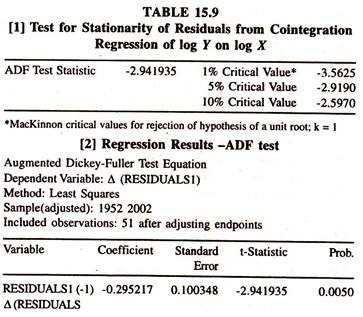
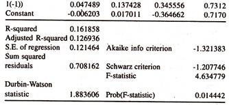
To find out the degree of integration of the residuals from the cointegration regression of exports on imports and imports on exports, ADF test statistic is estimated for residuals and furnished in tables 15.8 and 15.9. Table 15.10 [residuals of cointegration regression of log Y on log X] and table 15.11 [residuals of cointegration regression of log X on log Y] report the calculated ADF statistic for the level of the residuals obtained from the cointegration regression of exports on imports and imports on exports.

The calculated ADF statistics are higher than the MacKinnon critical values showing that the residuals in level form are on a stationary process i.e., they are I(0). The degree of integration of the residuals obtained from the two cointegration equations is less than the degree of integration of the variables used in estimating cointegration regression.

Therefore, though the exports and imports series are non stationary in log level form [Two variables individually are not mean reverting i.e., the deviation of the item of the variable (log Y or log X) from the mean value does not have a tendency to revert through time to the mean value], their linear combination [Residuals of [i] actual exports from the long run equilibrium path [log Y_t – (b₀ + b₁ log X_t)] and [ii] actual imports from the long run equilibrium path] [log X_t – (b₀ + b₁ log Y_t)] is stationary (errors are a zero mean reverting) in level form evincing the fact that exports and imports are co integrated in the long run.

This empirical content [through the Engel – Granger Representation] leads to conclude that there is a long run equilibrium relationship between exports and imports. In other words, exports and imports are not drifting farther from each other in the long run.

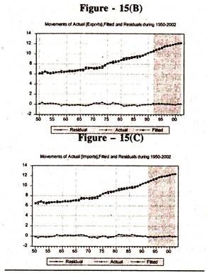
The figure 15(B) and figure 15(C) corroborate the fact that two variables [exports on imports and imports on exports] are co integrated as the residuals, deviations of actual values from the equilibrium path, are stationary around the zero mean values

 

Error Correction Modeling [ECM]:

Short Run Dynamic Adjustments towards Long Run Equilibrium:

Though exports and imports have a tendency to converge towards an equilibrium path in the long run [long run equilibrium between exports and imports] they may diverge from equilibrium path in the short run [short run disequilibrium between actual values of exports [in case of the exports on imports] and long run equilibrium values or actual values of imports[in case of imports on exports] and long run equilibrium values .

The disequilibrium between short run and long run values in lagged year would be corrected/adjusted quickly or slowly in current year by the changes in exports or imports through the trade policies.

The ECM, which combines both long run cointegration relationship and short run corrections/adjustments of co integrated variables towards the long run equilibrium, is also attempted to first differenced variables and error correction variable, which are stationary. The data used are given in table 15.12. The results of the same are presented in Tables 15.13 and 15.14 respectively.

Further, the regression coefficients on log imports and log exports in two cointegration regression equations, constant elasticities, are close to unity, which will be expected in the long run.

The regression results based on ECM [Table 15.13 and Table 15.14] show that the coefficients on Δ log Y and Δ log X , [ derivative of fi-st differenced variable, exports or imports, with respect to first differenced variable, imports or exports] short run elasticities are significantly positive and less than the coefficients on log Y and log X [level variables], long run elasticities, in cointegration regression evincing the positive effect of additional unit of exports on imports and imports on exports in the short run. i.e. short run percentage effect.

The coefficient on Error Correction term [which gives an indication of short run deviations from the long run equilibrium][table 15.13] in ECM equation is negatively insignificant evincing the fact that the disequilibrium between short run values and long run values in lagged periods is neither corrected nor extended each period showing that there are no disturbances present.

In other words, the changes in exports adjust to the changes in imports in the same year. Thus, there is equilibrium both in short run and long run periods. In table 15.4, the coefficient on error correction term is negatively significant. This provides an important information on the short run relationship between exports and imports in India.

The estimate of coefficient of error correction term, known as constant elasticity, specifies that the changes in imports respond to a deviation from the long run equilibrium.

This shows that twenty six percent of disequilibrium in t-1 period is corrected in t period. Thus, though there is disequilibrium between short run and long run, about twenty six percent of the disequilibrium in t-1 period is corrected/ adjusted every year by the changes in imports.

Differential Coefficients of Error Correction Term:

The presence/absence of shift in the regression coefficients of error correction term can be scanned by fitting the ECM to data given in table 15.15

The results furnished in table 15.16 [[Δ logY on Δ log X, lagged error and dummy lagged error] show that the differential coefficient of error correction term is insignificant showing the absence of shift in the coefficient of error correction term [ECT] during post economic reform period[D = 1].

Therefore the sign and size of the coefficient of ECT will be the same both in the presence of attribute [post economic reform period] and absence of attribute [pre economic reform period].

It should be noted that the regression coefficient of ECT is also negatively insignificant showing the presence of equilibrium in the short run .Therefore it can be concluded that both in the absence [pre economic reform period] and presence [post economic reform period] there is a short run equilibrium.

The regression results given in table 15.17 show that the differential coefficient of error correction term is negative but not significant evincing the absence of shift in the coefficient of error correction term during post economic reform period. The regression coefficient of error correction term in the absence of attribute [pre economic reform period] is significantly negative showing the presence of short run disequilibrium .

The sign and size of the coefficient of error correction term in the absence of attribute would continue even in the presence of attribute. The policy variable [economic reforms] could not be able to bring any drastic change in reducing the disequilibrium when D = 1 .

It should be noted that in order to examine the differential intercept and differential coefficient of first differenced independent variable, both dummy variable and dummy times first differenced variables [Interaction variable] need to be included along with dummy times error correction term in ECM model.

If differential intercept and coefficient of dummy variable times first differenced variable are not significant then the ECM can be estimated with first differenced independent variable, lagged error term and dummy lagged error term.