
The below mentioned article provides a study note on the Engel function in economics.
Engel’s Laws:
The relationship between total consumption expenditure and expenditure on a specific item at a point of time across the sample households is known as Engel Function or Engel Curve.
The empirical results of the study undertaken by Engel [Ernst Engel was German Statistician] were published in 1895.The advantage of taking up cross-sectional studies is that the prices of the commodities will be constant across households at a point of time.
ADVERTISEMENTS:
Because of this, the relationship between total expenditure and expenditure on a specific item incurred by cross-sectional families would empirically be studied to examine consumption patterns. In other words the demand for specific items by cross-sectional families would be studied to examine the responsiveness of consumption expenditure on specific item to the changes in total expenditure.
According to Engel’s law “The proportion of total expenditure incurred on food items declines as total expenditure [which is proxy for income] goes on increasing.”
This law can be understood from the following table:
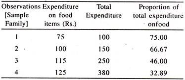
The number of items to be purchased in general go on increasing with an increase in income. If the level of income is low, then only one item will be purchased and the proportion of total expenditure incurred on the item will be constant. If income continues to rise additional items would be purchased by households. Then the proportion of total expenditure on the first item would gradually decline.
ADVERTISEMENTS:
The proportion of total expenditure on the item [which may be essential or luxurious] declines/increases or remains constant with the increase in total expenditure. Thus the variations in expenditure across households can be seen. Though the consumption expenditure on items goes on changing from household to household, the prices of the commodities facing the cross-section of households would generally be constant.
In economic analysis, the differences in the consumption patterns of households can be explained due to the variations in total expenditure, [which is the summation of the expenditure on food and non-food items.] Any variation in consumption patterns that is not explained by the changes in total expenditure can be attributed to non-economic factors such as the changes in taste.
One of the major reasons for such changes in taste is variations in family size. Therefore, there is a need to adjust for changes in the family size of households to capture the impact of family size along with other important independent variables on consumption expenditure.
ADVERTISEMENTS:
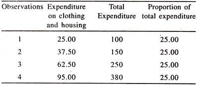
According to Engel’s second law, the proportion of total expenditure on clothing and housing will be approximately constant [stable] with the increase in total expenditure.
This law can be understood from the following table:
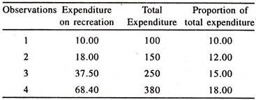
According to Engel’s third law, the proportion of total expenditure spent on recreation goes on increasing with the increase in total expenditure.
This law can be understood from the following table:
The relationship between total expenditure and expenditure on a specific item [food or non-food] is referred to as the Engel function or Engel’s law or Engel curve.
Engel’s function can be expressed as follows:
Y = f [X]
ADVERTISEMENTS:
Where,
Y= expenditure on specific item-[food or non-food item]
X- total expenditure [proxy for income]
The change in Y due to the change in X for a specific item is referred to as Marginal Propensity to Consume. This is also known as marginal effect.
ADVERTISEMENTS:
The responsiveness of Y to the changes in X is referred to as the elasticity of Y with respect to X, known as Engel Elasticity. Sometimes, the sign and size of the Engel elasticity will be considered for classifying the goods/commodities into necessities, luxuries etc.,
Forms of Engel Curves:
In econometric works, Engel Elasticities are estimated by fitting different forms of regression equations [Engel Curves], to cross section data.
The most important forms of regression models [Engel Functions] in the empirical studies are:
ADVERTISEMENTS:
1. Linear
2. Semi-log
log of Y on X
Y on log X
3. Power function
or log-linear
ADVERTISEMENTS:
or double log
or constant elasticity model
4. Quadratic
5. Cubic
6. Inverse
7. Log-inverse
ADVERTISEMENTS:
The Linear Regression Model:
The specification of a simple linear [first degree i.e. Y = b0 + b1 X1 + error] form of engel function will be as follows:
Y = b0 + b1 X + error (1)
The derivative [How the dependent variable (Y) changes for a small change in the independent variable (X)] of Y with respect to X, dY/dX is b1, which is marginal propensity to consume. This will be constant and less than unity.
The Engel Elasticity [ey.x] will be evaluated at the mean [average] values of Y and X as follows:
ey.x = dY/dX* Mean of X/Mean of Y
ADVERTISEMENTS:
= b1 * Mean of X/Mean of Y
Therefore, this value is referred to as an average elasticity of Y with respect to X. Sometimes the Engel Elasticity will be evaluated at different values of X and Y. Therefore the elasticity estimated from linear regression model will be variable. If the value of eY.X is more than unity then Y/X [Ratio of expenditure on ith item to total expenditure] goes on increasing with the increase in total expenditure.
If it is less than unity then Y/X goes on declining with the increase in total expenditure. If it is unity then the ratio of Y to X [Y/X] will be constant with the increase in total expenditure. The Engel Elasticity will be directly related to the increase in total expenditure, all else equal and inversely related to the increase in expenditure on ith item, all else equal.
If the linear form of regression equation [Linear engel curve] is not found suitable to the cross section observations then the other forms of regression equations [models] have to be fitted. Of different forms of regression equations [Engel curves], the semi-log form of regression is widely fitted to the cross-section data.
Semi Log Regression Model:
The specification of a semi log [One of the two variables [Y or X] will be in log form] form of engel function will be as follows:
ADVERTISEMENTS:
[i] log Y = b0 + b1X………. (2)
The derivative of log Y with respect to X
[d log Y/ dX = dY/ Y/dX/ 1 = dY/dX* 1 / Y], b1 shows the proportionate change in Y for a unit change in X.
The rate of change in Y per a unit change in X,
dY / dX = b1Y, is an mpc [marginal effect]
The Engel Elasticity from this function will be estimated as follows:
eY.X = dY / dX * X/Y = b1Y. X / Y = b1X
Thus, an mpc is the independent of the changes in X and elasticity is independent of changes in Y. Therefore, both mpc and engel elasticity are variable in the regression model of log Y on X.
[ii] Y = b0+ b1 log X…………….. (3)
The derivative of Y with respect to log X,
[dY / d log X = dY / 1 / dX / X = dY / 1 / dX / X = dY / dX / X / 1] , b1, shows the the rate of change in Y per a proportionate change in X.
The rate of change in Y per a unit change in X [mpc] is:
dY / dX = b1/ X
The Engel Elasticity from this function will be estimated as follows:
e Y.X = dY / dX.X / Y = b1/ Y
Thus, both mpc and engel elasticity are variable.
If this form of regression equation to the cross sectional is not suitable then the other forms of equations have to be attempted.
Double Log Regression Model [Power Function]:
The Power function, Which is also known as double log or log linear or constant elasticity model, is popular in empirical studies as the regression coefficient of independent variable directly provide us constant Engel Elasticity, as shown below:
Y = b0 Xb1………………. (4)
The derivative of Y with respect to X,
dY/dX = b1 Xb1-1
= b1 b0 Xb1 X-1
= b1* b0 Xb1/X
= b1* Y/X, is an mpc which goes on changing with the change in Y or X.
The engel elasticity from this function is which is constant, as shown below:
dY / dX.X /Y = b1Y/ X.X/Y = b1
Thus, the Engel Elasticity is independent of changes in X and Y.
In order to estimate by OLS method, the above Power function will be transformed into log linear [known as double log] form as shown below:
log Y = log b0 + b1 log X……………. (5)
The derivative of log Y with respect to log X [known as engel elasticity],
dlog Y / dlog X = dY / Y /dX / X
= dY / Y.X / dX = dY / dX.X / Y, is b1
which is a constant. If this function is not found suitable to the cross-sectional data points, then the other forms of regression equations [Engel functions] have to be tried.
The other form of regression equation that can be fitted to the cross-sectional data to estimate Engel Elasticity is quadratic form of regression equation.
Quadratic Regression Model [Second Degree Polynomial Regression Model]:
The specification of a quadratic [Square of the independent variable [X] along with X is considered] form of engel function will be as follows:
Y = b0 + b1 X – b2 X2……………………….. (6)
Or
Y = b0 – b1 X + b2 X2………………………… (7)
The derivative of Y with respect to X,
dY / dX = b1– 2 b2 X 2-1
= b1 – 2 b2 X, is an mpc which goes on changing with the change in X. If the sign of regression coefficient of X, b1, is positive or negative then the regression coefficient of X 2, b2, will be negative or positive. Thus they have opposite signs.
The Engel Elasticity [eY.X] will be estimated as follows:
eY.X = dY / dX.X/Y = b1 – 2 b2X. X/Y
= b1X – 2 b2X2/Y
Thus the Engel Elasticity in the quadratic form of equation is also variable. If the signs of b, and b, are quite opposite [+ and – or – and +] then we get either an inverted ‘U’ shaped curve or a ‘U’ shaped curve.
If the quadratic equation is not found suitable to the cross sectional data points, then the other forms of regression models have to be attempted.
Cubic Regression Model [Third Degree Polynomial Regression Model]:
The specification of a cubic regression model [with higher powers of independent variable] will be as follows:
Y = b0 + b1 X – b2 X2 b3X3……………… (8)
The derivative of Y with respect to X (mpc) is,
dY/dX = b1 X1-1 – 2b2X2-1 + 3b3 X3-1
= b1 – 2b2 X + 3b3X2
The engel elasticity from this model will be estimated as follows:
ey.x = b1 – 2b2 X + 3b3 X2 . X/Y
= b1X – 2b2X2 +3b3X3. 1/Y
Inverse [Reciprocal] Regression Model:
The specification of an inverse [Independent variable [X] enters inversely [1/X or X-1] in the model] form of engel function will be as follows:
Y = b0 + b1 [1/X]
Or
Y = b0 + b1 X-1………… (9)
The derivative of Y with respect to X [mpc],
dY/ dX = (-1) b1 X -1-1 = – b1 X-2, is – b1/ X2
The engel elasticity from this model will be estimated as follows:
ey.x = dY/dX*X/Y = – b1/X2 / *X/Y = – b1/XY
If the sign of regression coefficient of 1/X,b1, is positive, then the signs of mpc and Engel Elasticity will be negative. If the sign of regression coefficient of 1/X,b1 is negative then the signs of mpc and Engel Elasticity will be positive.
If the inverse [reciprocal] regression model is not found suitable to cross sectional data, then the other forms of regression equations [Engel Functions] have to be attempted.
Log Inverse Regression Model:
The specification of a log inverse [Dependent variable [K] enters in log form and independent variable [X] enters in inverse form [1/X or X-1]] engel function will be as follows:
log Y = b0+ b1 1/X
or
log Y = b0 + b1 X-1 …………… (10)
The derivative of Y with respect to X [mpc] is:
d logY / dX = – 1. b1 X -1-1 = – b1 X-2
dY/Y.1 / dX = -b1 X-2
dY / dX 1/Y = – b1 X -2 = – b1/X2
dY / dX = – b1Y / X2
The engel elasticity from this model will be estimated as follows:
ey.x= dY / dX.X / Y = – b1Y / X2. X / Y = – b1 / X
Thus mpc varies with the change in X and Y and engel elasticity varies with the change in X only. In the case of log function also if the sign of regression coefficient of 1/X, b1, is negative or positive then the signs of mpc and elasticity will be positive or negative. So far as the simple engel function is concerned, the discussion is confined to estimating the elasticity of expenditure on ith item with respect to total expenditure only.
But in practice the total expenditure is not the only factor in influencing the expenditure on ith item, but also the family size.
Therefore both total expenditure and family size need to be considered as independent variables in the engel function [Multiple Engel function] to estimate the partial elasticities of expenditure on ith item with respect to total expenditure and family size [in male adult units]. In empirical studies both linear and double-log forms of engel curves are fitted to the cross sectional data.
The procedure required for estimating both marginal and percentage effects is explained below:
Multiple Linear Regression Model:
The specification of a multiple linear engel function [with two independent variables] will be as follows:
Y = b0 + b1 X1 + b2 X2 + e……………………. (11)
Where
Y = Expenditure on ith item
X1 = Total expenditure [Proxy for income]
X2 = Family size measured in male adult units
e = Random variable [error term with usual assumptions]
The partial derivative of Y with respect to X1 [keeping X2 constant],
∂Y/∂X1 = b1 is an mpc which is constant.
The partial derivative of Y with respect to X2 [Keeping X1 constant],
∂Y /∂X2, = b2 [constant] is the rate of change in Y per a unit change in X2 [keeping X1 constant]
The Engel Elasticities [eY.X1 and ey.X2] from a multiple linear regression will be calculated as follows:
The Partial elasticity of Y with respect to total expenditure,
ey x1= ∂Y/∂X1 . X1 /Y = b1* X1/ Y
The elasticity of Y with respect to family size,
ey X2= ∂Y/∂X2 . X2 /Y=b2* X 2/Y
In empirical studies the expenditure elasticities are being evaluated at mean values of Y, X1 and X2.
Therefore, the average elasticity of Y with respect to total expenditure will be as follows:
ey x1 = b1* mean of X1 / mean of Y
eY.x2 = b2* mean of X2/ mean of Y
If the linear regression equation doesn’t give good fit to the cross-section data, some other type of regression model has to be attempted.
Multiple log linear Regression Model:
In empirical studies, the power function, which is also identified as double-log, log-linear and constant elasticity regression model, is being widely used because the regression coefficients of independent variables [X1 and X2] directly give the constant elasticities.
The specification of a multiple power function will be as follows:
Y = b0 X1b1 X2b2……………… (12)
The partial derivative of Y with respect to X1 is
∂Y / ∂X = b1b0 Xb1-1 X2b2
= b1. b0 X b1 X2 b2 .X1-1
= b1 b0 X b1 X2 b2 .1/X1
= b1 Y/X1
This is referred to as an mpc and goes on changing with the changes in Y and X1.
The responsiveness of Y with respect to X1 which is the constant elasticity will be expressed as follows:
ey.x1 = ∂Y/∂X 1 X1/Y
= bxY / X1 X1/Y = b1
The partial derivative of Y with respect to X2 is
∂Y/∂X = b2b0X1b1 X2b2-1
= b2. b0 Xb1 X2 b2.X2-1
= b2b0 X1 b1 X2b2. 1/X2
= b2Y / X2
This is referred to as the rate of change in Y per a unit change in X2 and goes on changing with the changes in Y and X2.
The responsiveness of Y with respect to X2will be expressed as follows:
ey.x2 = ∂Y /∂X2*X2/ Y
= b2Y / X2. X2 / Y = b2 which is also constant.
For the purpose of estimation by Ordinary Least Squares method, the above power function is transformed into a log-linear model as follows:
log Y = log b0 + b1 log X1 + b2log X2 ………………. (13)
The partial derivative of log Y with respect to log X1
∂log y / ∂ log X1
= ∂Y/Y/∂X1/X1
= ∂Y/Y*X1/∂X1= ∂Y / ∂X1 . X1 / Y = b1,
is constant elasticity of expenditure on ith item with respect to total expenditure.
The partial derivative of log Y with respect to log X2,
d log y / d log X2
= dY / Y dX2 / X2
= dY / Y*X2 / dX2
= ∂Y/∂X2*X2/Y = b2,
is also constant elasticity of the expenditure on ith item with respect to family size. Thus, both in the power function and log linear model, the regression coefficients of total expenditure and family size are constant elasticities. One of the advantages of this model is that the sum of partial elasticities of expenditure with respect to total expenditure and family size gives an idea about the nature of economies of scale in consumption expenditure.
If the sum of b1 and b2 = 1, then there will be no economies of scale in consumption expenditure [Linear Homogeneous Engel Function], If the sum of b1 and b2 > 1, then there will be diseconomies of scale in consumption expenditure [Non-Linear Homogeneous Engel Function]. If the sum of b1 and b2 < 1, then there will be economies of scale in consumption expenditure [Non-Linear Homogeneous Engel Function].
No economies of scale imply that a one percent increase in total expenditure and family size leads to increase the expenditure on ith item by the same percent.
Diseconomies of scale imply that a one percent increase in total expenditure and family size leads to increase the expenditure on ith item by more than one percent.
Economies of scale imply that a one percent increase in total expenditure and family size leads to increase the consumption on ith item by less than one percent.
Per Capita Engel Function [Restricted Engel Function or Linear Homogeneous Engel Function]:
The problem of multicollinearity between total expenditure and family size is quite common. In order to avoid this problem to some extent the following per capita specification of Engel function will be considered in empirical studies.
[Y/X2] = b0 [X1 /X2]b1 ………………..(14)
For the purpose of estimation, the above regression model [power function] is transformed in to a log linear form as shown below:
log [Y1/X2] = log b0 + b1 log [X1/X2]
log Y – log X2 = log b0 + b1 log X1 – b1 log X2
log Y = log b0 + b1 log X1 – b1 log X2 + log X2
= log b0+ b1 log X1 + [1-b1] log X2
= log b0 + b1 log X1 + b2 log X2
1 – b1 = b2
1 = b2 + b1
If no economies of scale occur [∑(b1 + b2) = 1] then the above per capita specification will be preferred to the multiple log- linear regression model. One of the advantages of the per capita specification is that the degree of problem of multi collinearity can to some extent be reduced. If no economies of scale do not occur, then the regression model based on per capita specification will not be appropriate to cross-section data.
In order to allow for the presence of economies of scale and diseconomies of scale in consumption expenditure, the multiple log-linear function will be preferred. It should be noted that the above per capita specification is used only if the sum of expenditure elasticities on ith item with respect to total expenditure and family size is unity.
Apart from the above two independent variables, family size and total expenditure, the other variables such as age of head of the family, education of the head of the family etc., may also be included in the Engel function to capture their impact on the consumption expenditure on ith item.
Log Linear Engel Function with an Interaction Variable: Differential Engel Elasticity:
The impact of qualitative variable such as region, caste education etc., along with a quantitative independent variable may also be scanned on the expenditure on ith item by introducing an interaction variable (product of dummy variable [Proxy for qualitative variable] and quantitative independent variable i.e., total expenditure) with the following specification.
log Y = log b0 + b1 D + b2 log X + b3 [D *log X]………….. (15)
Where
Y = Expenditure on ith item [Food or non-food items]
X = Total expenditure on food and non food items
D = Dummy variable, which is proxy for qualitative variable such as education, region, caste etc., would take 1 in the presence of the attribute and 0 in the absence of attribute.
When D = 1, then the log linear [engel function] regression model will be as follows:
log Y = [b0 + b1] + [b2 + b3] log X ……………….(16)
Where
The derivative of log Y with respect to log X is, ∂ log Y/ ∂ log X, is the constant engel elasticity, [b2+ b3], in the presence of attribute.
b3 is the differential Engel elasticity when D = 1
is the differential intercept when D = 1
When D = 0,then the log linear [engel function] regression model will be as follows:
log Y = b1 + b2 log X…………………….. (17)
The derivative of log Y with respect to log X, ∂ log Y/ ∂ log X, is the engel elasticity [b2] in the absence of attribute [D = 0], When D = 1, if b3 is significantly positive, then the size of engel elasticity will be higher in the presence of attribute as compared to the size of engel elasticity in the absence of attribute. If b3 is significantly negative then the size of engel elasticity will be lower as compared to the size of engel elasticity in the absence of attribute.
If b3 is statistically not significant then the size of engel elasticity will be identical [stable or homogenous] both in the presence and absence of the attributes. This regression equation [model] would be common in the presence and absence of attribute. Thus, an interaction variable in the engel function will be useful in scanning the shift in the magnitude [degree] of engel elasticity.
Therefore, in the empirical studies an interaction variable can be considered in the set of independent variables. With the advent of software packages on econometrics, the different forms of engel functions can easily be fitted to the cross-section data. The choice of the engel function for the analysis depends on economic, statistical and econometric criteria.
The economic criterion is concerned with the sign and size of the engel elasticity. The statistical criterion is concerned with statistical significance of the regression coefficients of independent variables and goodness of fit. The econometric criterion is concerned with mainly the problem of heteroscedasity as cross sectional data will be used to estimate engel elasticities.
Linear Engel Function and Adding Up Criterion:
One of the advantages of fitting the linear simple regression model for food and non food items is that it satisfies the adding-up criterion that the sum of the expenditure incurred on all items should be equal to total expenditure [Total expenditure (proxy for income) will be exhausted if it is incurred on both food and non food items]
If two linear regression equations for food and non-food items are fitted to cross section data then the equations will be as follows:
Yr = b0 + b1 X……………… (18)
Ynf = c0 + c1 X…………….. (19)
Where
Yf = Expenditure on food items
X = Total expenditure [sum of food expenditure and non food expenditure that is ∑ (Yf + Ynf)] which is the independent variable in two equations
Ynf = Expenditure on non-food items
The sum of the numerical values of b1 and c1 [constant marginal propensities to consume for food and non-food items respectively] will always be equal to unity as the expenditure incurred on food and non food items will be equal to total expenditure.
It should be noted that the degree of reliability of mpc and engel elasticities is directly associated with the increase in cross-section observations. Then the estimates of parameters of mpc and engel elasticities will be close approximates to the true parameters.
Engel Functions—Estimates of Economic Relationships:
The following data [Table 2.1] on monthly consumption expenditure and total expenditure in rupees collected from twenty-five sample households are considered for estimating the engel elasticities by fitting different forms of engel functions.


Where,
1. R 2 = [Explained variation/Total variation] =
∑(Trend values of Yi – Mean value of Y)2 = / ∑(Actual values of Y – Mean value of Y)2
2. Sum of squares of residuals = ∑ (Actual values of Y – Trend values of Y)2 = ∑ei2
3. Standard error [S.E.] of regression = Square root of ∑ei2/n-k
4. Durbin-Watson Statistic (d) = ∑(et – et-1)2 /∑et2
The results of the simple linear engel function [Table 2.2] fitted to the cross section data show that the regression coefficient of total expenditure is significantly positive.
This explains that the rate of change in consumption expenditure on food items per unit change in total expenditure [Marginal Propensity to Consume] is less than unity. Out of this estimate it can be inferred that a one unit increase in total expenditure leads to increase the consumption expenditure on food items by 0.87 units. This value is in line with the theory.
The average engel elasticity estimated at the mean values of Y and X [regression coefficient times the ratio of the mean value of X to the mean value of the Y : 0.871705*3820.840/3383.920] is 0.984. Out of this value it can be inferred that a one percent increase in total expenditure leads to increase the consumption expenditure on food items by 0.984 per cent [which is close to unity], all else equal.


The results of the log linear engel function [Table 2.4] fitted to the cross section data [Table 2.3] show that the regression coefficient of log total expenditure is significantly positive and unity.
That is 1.002. This is known as constant engel elasticity of expenditure on ith item with respect to total expenditure. It can be inferred from this that a one percent increase in total expenditure leads to increase the consumption expenditure on food items by 1.02 per cent [which is approximately unity], all else equal.

The results of the semi log regression model [Table 2.5] fitted to the cross section data [Table 2.3] show that the regression coefficient of total expenditure is significantly positive and its value is 0.000272.
This explains that the proportionate change in Y per unit change in X is 0.000272.The mpc [estimated at mean value of Y :0.000272*3383.90] is less than unity that is 0.92. The Engel elasticity, which is 1.039 [0.000272 * 3820.840 = 1.039], explains that a one percent increase in total expenditure leads to increase the consumption expenditure by 1.039 percent.
The results of the semi log regression model fitted to the cross section data [Table 2.6] show that the regression coefficient of log total expenditure, the rate of change in Y per a proportionate change in X [b1] is significantly positive i.e., 3054.553.
The value of mpc is less than unity that is 0.7994 [3054.553/3820.840], The Engel elasticity, which is 0.9027, [estimated at mean value of Y:3054.553/3383.920] explains that a one percent increase in total expenditure leads to increase the consumption expenditure on ith item by 0.9027 percent.

The results of the inverse regression model [Table 2.8] based on the data given in table 2.7 show that the regression coefficient of MX is negatively significant. The mpc [estimated at the square of the mean of X:dY/dX = -b1 /X2= 7604940/ (3820.840)2 = 0.5] less than unity. The Engel elasticity is 0.588 [estimated at the product of mean values Y and X:7604940/ [3383.920*3820.840].
Out of this, one can infer that a one percent increase in total expenditure leads to increase the consumption expenditure on food items by 0.588 percent. It should be noted that both mpc and engel elasticity estimated from the inverse regression model are relatively smaller as compared to the estimates emerged from other models.
The results of the log inverse regression model [Table 2.10] based on the data given in table 2.9 show that the regression coefficient of 1/X is negatively significant. The mpc [estimated at the square of mean of X and mean of Y:2715.653*3383.920)/(3820.840)2 = 0.62947] is less than unity.
The elasticity [estimated at the mean value of X:2715.653/3820.84 ] is 0.717148. Out of this one can infer that a one percent increase in total expenditure leads to increase the consumption expenditure on food items by 0.717048 percent, all else equal.
 The results of the quadratic regression model [Table 2.12] based on the data given in table 2.11 show that the regression coefficient of X is positively significant at one percent level and that of X 2 is moderately significant.
The mpc estimated [1.037 – (2*0.0000185*3820.84)] is 0.8956. The estimated Engel elasticity is 1.011, which is close to unity. Out of this one can infer that a one percent increase in total expenditure leads to increase the consumption expenditure on food items by 1.17 percent.

The data points given in table 2.13 are used to prove that the linear engel function satisfies the adding up criterion.
The regression results of the linear engel functions fitted for food [Table 2.14] and non food [Table 2.15] items show that the sum of constant mpc for food items and constant mpc for non food items [0.871705 + 0.128295] is equal to unity satisfying the adding up norm.


The choice of the regression results of Engel function for the analysis, policy making and forecasting depends on economic, [Sign and size of the coefficients] statistical [Standard errors and goodness of fit] and econometric [Assumptions of OLS method] criteria.
Multiple and Per Capita (Linear and Log linear) Engel Functions:
In order to estimate the multiple Engel function [both linear and log linear forms] the following cross section data Monthly Expenditure on food items, Family size and Monthly total expenditure are used.
The regression results of multiple linear Engel model based on the data given in table 2.16 are presented in table 2.17.

The regression results show that the coefficient of monthly total expenditure is highly significant and positive and the coefficient of the family size is also positive but moderately significant .Thus the two variables included in the linear regression model are influencing the monthly consumption expenditure on food items. The partial elasticity of Y with respect to X1 [ey.x1] , keeping X2 constant, is 0.88 showing that the average elasticity is less than unity.
The partial elasticity of Y with respect to X2 [ey.x2 ], keeping X1 constant, is 0.14 showing that the average elasticity is very stumpy. It should be noted that the two independent variables, X1 and X2, move together in the same direction leading to the problem of multicollinearity [correlation between X1 and X2] The degree of correlation between XI and X2 can be assessed through the values furnished in table 2.18.

The degree of correlation between X1 and X2 is very soaring showing the presence of high multicollinearity between them. In order to avoid the problem of multicollinearity the per capita expenditure variables [ratio variables: Y/X2 and X1/X2] have been considered. The data points on per capita variables are generated and furnished in table 2.19. The regression results of the per capita engel function are given in table 2.20


The regression results [ table 2.20] based on per capita specification show that the regression coefficient of monthly per capita total expenditure is positively significant showing that a one unit increase in total per capita expenditure is associated with the increase of 0.86 units in monthly per capita expenditure on food items The average elasticity of per capita expenditure with respect to per capita total expenditure [e Y/x2 x1/x2 ] is 0.97.
It should be noted that the per capita specification can be considered only if there are economies of scale in consumption expenditure despite the fact that there is an advantage of avoiding the problem of multicollinearity between two independent variables. The data given in table 2.16 are considered for fitting the multiple log linear engel function by OLS method. The regression results of the same are given in table 2.21.

The regression results show that the coefficient of total expenditure, constant elasticity of Y with respect to X1, is positively significant and close to unity. The coefficient of family size, constant elasticity of Y with respect to X2, is positive but not significant. In the log linear multiple Engel function the coefficient of family size is positively insignificant. One of the likely reasons for such a perplexing result is the presence of sturdy correlation between X1 and X2 [Table 2.22].

Keeping the evidence of sturdy correlation between X1 and X2 [0.91] in view, the data on log per capita variables are generated [Table 2.23] for fitting per capita engel function. The regression results of the same are presented in table 2.24


The results based on the regression of per capita expenditure on per capita total expenditure [Table 2.24] show that the elasticity of per capita consumption expenditure on food items with respect to per capita total expenditure is positively significant and approximately unity thereby showing that a one percent increase in per capita consumption expenditure on food items leads to increase the per capita consumption expenditure by one percent.