The below mentioned article provides a study note on the marketed surplus function.
In order to examine the responsiveness of marketed surplus of food grains to the changes in quantity of production of food grains the following regression models are considered in empirical studies:
Linear Marketed Surplus Function:
Specification of the linear Marketed Surplus Function will be as follows:
Y = b0 + b1X + error……………… (111)
ADVERTISEMENTS:
Where
Y = Quantity of marketed surplus of food grains
X = Quantity of production of food grains
b0 is the quantity of marketed surplus [Deficit or Surplus] in the absence of production
ADVERTISEMENTS:
b1 is marginal propensity to sell i.e., dY/dX, whose value will always be positive.
The numerical values of b0 and b1 will be estimated by Ordinary Least Squares method with specific assumptions.
The elasticity of marketed surplus of food grains with respect to production of food grains [eY.X = dY/dX. X/Y] will be estimated as follows:
eY.X = b1. mean of X/mean of Y
ADVERTISEMENTS:
The mean value of X and Y or total values of X and Y or the individual values of X and Y [elasticity varies from point to point], will be considered to evaluate the elasticity of marketed surplus of food grains with respect to production [output elasticity of marketed surplus of food grains]. In empirical studies, the mean values of X and Y will be used.
.Therefore, the elasticity is referred to as an average elasticity of production of marketed surplus of food grains. Apart from the linear marketed surplus function, the log linear form of marketed surplus function will also be considered in empirical studies.
Log Linear Marketed Surplus Function:
Specification of a log linear Marketed Surplus Function will be as follows:
log Y = log b0 + b1 log X ……………….(112)
The above function will also be estimated by OLS method. The derivative of log Y with respect to log X, d log Y/d log X, is b1. This value directly gives the numerical value of production [output] elasticity of marketed surplus [constant elasticity of marketed surplus with respect to production]. On the basis of size of b1, [more than unity or less than unity or unity,] the degree of responsiveness of marketed surplus to the changes in production can be understood.
The linear and log linear forms of marketed surplus functions will be estimated using cross sectional farm data [The data collected will be related to a single agricultural year] Apart from the variable of production, other variables such as the area under the crop, family size, prices of the crop concerned will also be considered.
It should be noted that the movement of the two variables either in the same direction or opposite direction creates a problem of multicollinearity. The problem of multicollinearity in marketed surplus function can be examined through the correlation matrix [correlation coefficients between the independent variables].
If the problem multicollinearity is found to be serious, then the degree of correlation between the independent variables can be reduced or eliminated either by deleting unimportant variables or taking ratio variables [such as per capita or per acre variables]. Further it should be noted that the variations in the farm prices at a point of time [since cross sectional farm data are used] will be constant.
Therefore the impact of prices on the marketed surplus of food grains using cross sectional farm data cannot be captured. Therefore the impact of prices on the marketed quantity [market arrivals: the quantity actually sold in the regulated agricultural markets] or marketed surplus [expost concept] can be scanned using the time series data.
ADVERTISEMENTS:
Then the following forms of regressions will be used:
(a) Linear Market Arrivals Function
(b) Log Linear Market Arrivals Function
Linear Market Arrivals Function:
Specification of a linear Market Arrivals Function will be as follows:
ADVERTISEMENTS:
Y = b0 + b1X + error ……………(113)
Where
Y = Quantity of Market Arrivals [quantity actually sold in a regulated agricultural markets] of food grains
X = Average Price of a Crop [food grains]
ADVERTISEMENTS:
b0 is the quantity of market arrivals [technically trend value] in the absence of prices
b1 is the derivative of Y with respect to X i.e., dY/dX, whose value will always be positive.
The values of b0 and b1 in the market arrivals function will be estimated by Ordinary Least Squares method.
The elasticity of market arrivals of food grains with respect to average prices will be
eY.X = dY/dX. X/Y
ey.x= b1. X/Y
ADVERTISEMENTS:
The mean values of X and Y or total values of X and Y or the individual values of X and Y will be considered to evaluate the elasticity of market arrivals with respect to prices of food crop [Price elasticity of market arrivals]. In empirical studies the mean values of X and Y will be used.
Therefore, the elasticity is referred to as an average elasticity of market arrivals of food grains with respect to prices. Apart from the linear market arrivals function, the log linear form of regression equation will also be considered in empirical studies.
Log Linear Market Arrivals Function:
The Specification of a log linear market arrivals function will be as follows:
log Y = log b0 + b1 log X……………. (114)
The above function will also be estimated by OLS method. The derivative of log Y with respect to log X, d log Y/d log X is b1. This value directly gives the numerical value of the elasticity of market arrivals with respect to the prices. On the basis of the value of b1, whether it is more than unity or less than unity or equal to unity, the degree of responsiveness of market arrivals to the changes prices can be examined.
Marketed Surplus Function- Estimates of Economic Relationships:
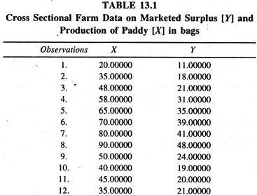
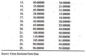
The cross sectional farm data given in Table 13.1 are considered for estimating the linear marketed surplus function.
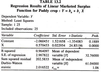
The regression results of the linear marketed surplus function [Table 13.2] illustrate that the regression coefficient of output of paddy, constant marginal propensity to sell [dY/dX], is appreciably positive.
The elasticity of marketed surplus with respect to output of paddy [estimated at the mean values of Y and X :0.57 * 61.04/32.76)] is a little above the unity showing that a one percent increase in the production of paddy leads to increase the marketed surplus quantity by 1.06 percent, all else equal. The negative sign of the intercept shows the deficit in the marketed surplus in the absence of production. In other words the minimum level of retention is higher.
ADVERTISEMENTS:
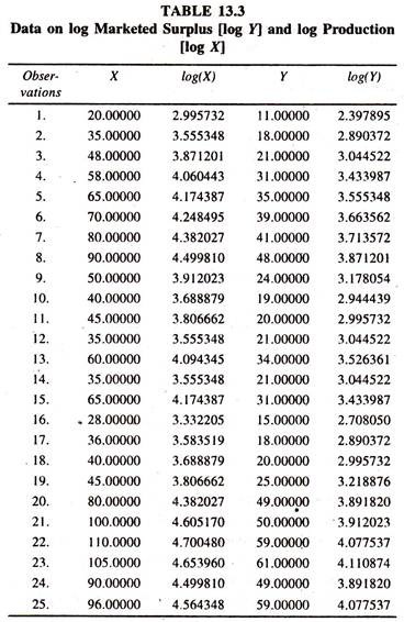
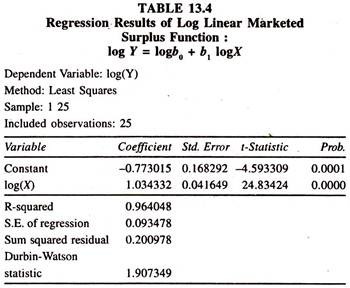
The data [Table 13.3] on log marketed surplus [7] and log production of paddy have been used to fit the log linear marketed surplus function. The regression results of log linear marketed surplus function for paddy crop [Table 13.4] show that the regression coefficient of output of paddy, which is constant output elasticity of marketed surplus, is significantly positive.
The value is just above the unity ,as in the case of linear marketed surplus function, showing that a one percent increase in output of paddy leads to increase the marketed surplus of paddy by 1.034 percent, all else equal.
