Risk: Meaning, Types and Measurement | Firm

In this article we will discuss about:- 1. Meaning of Risk 2. Types of Risk 3. Measurement.

Meaning of Risk:

By the term risk we mean a situation in which the possible future outcome of a present decision is plural and in which the probabilities and dimensions of their outcomes are known in the form of a frequency distribution. Risk refers to variability. It is measured in financial analysis generally by standard deviation or by beta coefficient. Technically risk can be defined as a situation where the possible consequences of the decision that is to be taken are known.

Risk is composed of the demands that bring in variations in return of income. The main forces contributing to risk are price and interest. Risk is also influenced by external and internal considerations. External risks are uncontrollable and broadly affect the investments.

These external risks are called systematic risk. Risk due to internal environment of a firm or those affecting a particular industry are referred to as unsystematic risk. Unsystematic risk is unique to a firm or industry. It does not affect the investor. Unsystematic risk is caused by factors like labour strike, irregular disorganised management policies and consumer preferences.

Types of Risk:

1. Systematic Risk:

Market risk, interest rate risk and purchasing power risk are grouped under systematic risk.

They are explained as under:

(i) Market Risk:

It is referred to as stock variability due to changes in investor’s attitudes and expectations. The investor’s reaction towards tangible and intangible events is the chief cause affecting market risk. Market risk cannot be eliminated but it can be reduced. Market risk includes such factors as business recessions, depressions and long term changes in consumption in the economy.

(ii) Interest Rate Risk:

There are four types of movements in prices of stocks in the market. These may be termed as long term, cyclical, intermediate and short term. Traditionally, investors could attempt to forecast cyclical savings in interest rates and prices merely by forecasting ups and downs in general business activity.

The effect of interest rate can be different for lending institution and borrow­ing institution. In India, a combination of factors have produced a situation where it is difficult to accurately find out the changes in interest rates.

(iii) Purchasing Power Risk:

It is also known as inflation risk. It arises out of changes in the prices of goods and services and technically it covers both inflation and deflation periods. In India, purchasing power risk is associated with inflation and rising prices. All investors should have an approximate estimate in their minds before investing their funds of the expected return after making an allowance for purchasing power risk.

2. Unsystematic Risk:

It arises out of the uncertainty surrounding a particular firm or industry due to factors like labour strike, consumer preferences and management policies.

The two kinds of unsystematic risks in a business organisation are business risk and financial risk which are explained below:

(i) Business Risk:

Every firm has its own objectives and aims at a particular gross profit and operating income. It also hopes to plough back some profits. Business risk is also classified into internal business risk and external business risk. Internal business risk may be represented by a firm’s limiting environment within which it conducts its business. External risks are due to many factors and some of the important factors are business cycle, demographic factors, political policies, monetary policy and the economic environment of the economy.

(ii) Financial Risk:

It is associated with the method through which it plans its financial structure. If the capital structure of a company tends to make earnings unstable, the company may fail financially. Large amounts of debt financing also increase the risk. Financial risk can be stated as being between Earnings before Interest and Taxes, and Earnings Before Taxes.

Measurement of Risk:

A number of techniques have been suggested by economists to deal with risk in investment appraisal.

Some of the popular techniques used for this purpose are as follows:

1. Risk Adjusted Discount Rate Method:

This method calls for adjusting the discount rate to reflect the degree of the risk of the project. The risk adjusted discount rate is based on the presumption that investors expect a higher rate of return on risky projects as compared to less risky projects.

The rate requires determination of (i) risk free rates and (ii) risk premium rate. Risk free rate is the rate at which the future cash inflows should be discounted. Risk premium rate is the extra return expected by the investor over the normal rate.

The adjusted discount rate is a composite discount rate. It takes into account both time and risk factors.

Illustration:

A project with an outlay of Rs. 4,00,000, its risk adjusted discount rate is estimated at 18 per cent. The data on cash flow is as follows:

Should the project be accepted or rejected?

Accept the project: if NPV > 1

Reject the project: if NPV < 1

Using the risk adjusted discount rate we find that

2. The Certainty Equivalent Approach:

According to this method, the estimated cash flows are reduced to a conservative level by apply­ing a correction factor termed as certainty equivalent coefficient. The correction factor is the ratio of riskless cash flow to risky cash flow.

The certainty equivalent coefficient which reflects the management’s attitude towards risk is

Certainty Equivalent Coefficient = Riskless Cash Flow/Risky Cash Flow

Example:

A project is expected to generate a cash of Rs. 40,000. The project is risky but management feels that it will get at least a cash flow of Rs. 24,000. It means that certainty equivalent coefficient is 0.6.

Under the certainty equivalent method the net present value is calculated as:

Where

α_t = Certainty Equivalent Coefficient

A_t = Expected Cash Flow for year t

I = Initial outlay on the project

i = Discount rate

Illustration:

Pioneer Concern is considering a project with initial outlay of Rs. 18,00,000 with a risk free discount rate of 1.05 per cent. The expected cash flow and certainty equivalent coefficient are given below. What is NPV of the project?

3. Sensitivity Analysis:

The future is not certain and involves uncertainties and risk, the cost and benefits projected over the lifetime of the project may turn out to be different. This deviation has an important bearing on the selection of a project.

If the project can stand the test of changes in the future, affecting costs and benefits, the project would qualify for selection. The technique to find out this strength of the project is covered under the sensitivity analysis of the project. This analysis tries to avoid over estimation or underestimation of the cost and benefits of the project.

In sensitivity analysis, we try to find out the critical elements which have a vital bearing on the costs or benefits of the project. In investment decision, one has to consider as many elements of uncertainty as possible on costs or benefits side and then arrive at critical elements which effect the expected costs or benefits of the project.

How many variables should be tested to carry out the sensitivity analysis in order to find out its impact on costs or benefits of the projects is a matter of judgement. In sensitivity analysis, one has to consider the changes in the various factors correlated with changes in the other. In order to arrive at the degree of uncertainty, the decision maker has to make alternative calculation of costs or benefits of the project.

Sensitivity analysis is a simulation technique in which key variables are changes and the resulting change in the rate of return is observed. Some of the key variables are cost, prices, project life, market share, etc.

Usually this analysis provides information about cash flows under the assumptions:

(i) Pessimistic,

(ii) Most likely, and

(iii) Optimistic.

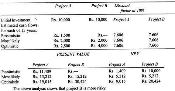
It explains how sensitive the cash flows are under these three different situations. If the differ­ence is larger between the optimistic and pessimistic cash flows, the more risky is the project.

Illustration:

Pioneer Company Ltd. is attempting to evaluate two projects A and B. Each project requires a net investment of Rs. 10,000 and the annual cash flows from each of the project is estimated at Rs. 2,000 p.a. in the next 15 years. The company’s cost of capital may be taken at 10%. In order to arrive at a decision about the selection of the project, the following data have been ascertained regarding the NPV of cash flows of each project.

4. Probability Theory Approach:

Yet another method for dealing with risks is to estimate the value for a result. Each value of prospective result is assigned a probability. Here one has to see a range of possible cash flows from the most optimistic to the most pessimistic for each pertinent year. Probability means the likelihood of happening an event.

It may be objective or subjective. An objective probability is based on a large number of observations under independent and identical conditions repeated over a period of time. A subjective probability is based on personal judgement. In capital budgeting decisions the probabilities are of a subjective type since they are based on a single event.

Process of Assigning Probabilities:

Here let us see the process of assigning probabilities.

It is subject to certain rules and they are:

(i) List of events collectively expansive

(ii) Events must be mutually exclusive

(iii) The numerical probabilities must add up to 1.

Basic Probability Theorem:

We must see certain basic theorems relating to a probability theory.

These are as follows:

(i) The probability of an event is always a number between 0 and 1 inclusive. If an event is sure to occur, its probability is by definition equal to 1. If it is certain that it will not occur its probability is 0.

(ii) If ‘n’ events are equally likely and only one of them may happen, then the probability of that event is 1/n.

(iii) If two events are mutually independent and the probabilities of one is PI while that of other P2, the probability of the events occurring together is the product of P1, P2.

(iv) If the events are mutually exclusive and the probability of the one is PI while that of the other is P2, the probability of either one or the other occurring is the sum P1+P2.

Illustration:

Pioneer Company Ltd. has given the following possible cash inflows for two of their projects A and B. Both the projects will require an equal investment of Rs. 5,000. Let us compute expected monetary values for the projects A and B.

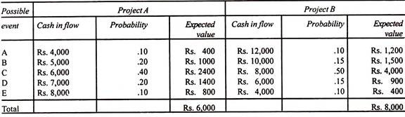
The above table shows that Project B has higher monetary value as compared to Project A. Therefore, Project B is preferable.

5. Standard Deviation:

Subjective judgment of the decision makers plays a crucial role in practice to resolve the prob­lem which may turn out to be imprecise or biased. There is no precise way to find the probabilities of different outcomes. This limitation is overcome by adoption of standard deviation approach.

The standard deviation is defined as the square root of the mean of the squared deviations of all the items from the mean and it is usual to denote it by the small Greek “Sigma”, σ. In the case of capital budgeting, this measure is used to compare the variability of possible cash flows of different projects from their respective mean or expected values.

Steps to be followed for calculating the S.D. of the possible cash flows:

(i) Compute the mean value of the possible cash flows.

(ii) Find out the deviation between the mean value and the possible cash flows.

(iii) Square the deviations.

(iv) Multiply the squared deviations by the assigned probabilities to get the weighted squared deviations.

(v) The sum of the weighted squared deviations and their square root are calculated. The result gives the S.D.

Illustration:

On the basis of the data given in probability theory approach find out which project is more risky by adopting S.D. approach.

A project having a larger standard deviation will be more risky as compared to a project having smaller standard deviation. In the above illustration, the standard deviation for project A is 1,095 while that of project B is 2,098. Hence project B is more risky.

6. Coefficient of Variation:

Standard deviation is expressed in the units of the original distribution and is called absolute measure of dispersion. Therefore, absolute measure must be reduced to a form which is free from the original unit of measurement. This can be done by expressing it in relation to the average from which variation is measured. This measure of relative variation is obtained by dividing the absolute measure by that average and is called a coefficient of variation.

The co-efficient of variation can be calculated as follows:

Coefficient of Variation = Standard Deviation/Expected (or Mean) Cash Flow = σ/Erf

On the basis of the data given in the standard deviation approach, the standard deviation for project A is 1095, while that for project B is 2098. The coefficient of variation of project B is more as compared to project A. Hence project B is more risky.

7. Decision Tree Analysis:

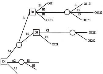
The decision tree analysis is another technique which is helpful in tackling risky capital invest­ment proposals. A decision tree is a graphic display of various decision alternatives and the sequence of events as if they were branches of a tree.

In constructing a tree diagram, it is a convention to use the symbol □ to indicate the decision point and O denotes the situation of uncertainty or event. Branches coming out of a decision point are nothing but representation of immediate mutually exclusive alternative options open to the decision maker.

Branches emanating from the event point ‘O’ represent all possible situations. These events are not fully under the control of the decision maker and may represent some other factors. The basic advantage of a tree diagram is that another act subsequent to the happening of each event may also be represented. The resulting pay-off for each act-event combination may be indicated in the tree diagram at the outer end of each branch.

Construction of Decision Tree:

The construction of a decision tree requires definition of proposal, identification of alternatives, graphing the decision tree, forecasting cash flows, and evaluating results.

This process can be under­taken in the following way:

(i) The first step in the construction of the decision tree is the definition of proposal. It means what is exactly required under the proposal.

(ii) The second step in the decision tree is the identification of alternatives. Each proposal will have at least two alternatives—accept or reject. In some cases, there may be more than two alternatives too.

(iii) The third step is graphing the decision tree. Decision tree is a graphical method. It visually helps the decision maker view his alternatives and outcomes.

Illustration of a Decision Tree Diagram:

(iv) The fourth step is forecasting cash flows. The forecasted cash flows regarding each decision branch are also shown along with the branch. Probabilities are also assigned to each cash flow. The probabilities of each event will be different.

(v) The fifth step in construction of a decision tree is evaluating results. The evaluation will be based on manager’s own experience, consultation with others and information available in this respect. On the basis of the expected value for each decision, the results are analysed. The firm may proceed with profitable alternative.

The pay-off for ultimate alternatives has been calculated by taking into account the probabilities of the ultimate alternative as well as for the previous alternative and multiplied by the expected pay-off of the first alternative without its probability. By incorporating probabilities of various events in the decision tree, it is possible to comprehend and trace probability of a decision leading to results desired.

What is significant about the decision tree approach is that it does several things for decision makers. It is highly useful to a decision maker in multi-stage situations which involve a series of decisions each dependent on the preceding one. It makes possible for them to see at least the major alternatives open to them and that the subsequent decisions may depend on events of the future.