Capital Budgeting: Meaning, Steps and Methods (With Diagram)

In this article we will discuss about the Capital Budgeting:- 1. Meaning of Capital Budgeting 2. Importance of Capital Expenditure to the Aggregate Economy 3. Central Role of Corporate Strategy and Capital Budgeting 4. Steps 5. An Overview 6. Methods Used to Make Investment Decisions 7. Capital Budgeting under Risk and Uncertainty.

Contents:

1. Meaning of Capital Budgeting 
2. Importance of Capital Expenditure to the Aggregate Economy 
3. Central Role of Corporate Strategy and Capital Budgeting 
4. Steps in Capital Budgeting
5. An Overview of Capital Budgeting
6. Methods Used to Make Investment Decisions in Capital
7. Capital Budgeting under Risk and Uncertainty

---

1. Meaning of Capital Budgeting:

Expenditures of buildings, plant and equipment, known as capital expenditures, are major decisions for most companies. A considerable portion of mon­ey is involved in it. Moreover, the management time involved is also significant.

It is because in­vestment decisions, unlike production and sales de­cisions, are long term in nature. So the company’s future profitability is at stake. Therefore, the pro­cess of evaluating capital expenditures, known as capital budgeting, is extremely important.

Capital budgeting refers to the process of allo­cating cash expenditures to investment which have a life longer than the operating period — normally a year. In other words, capital budgeting, or capi­tal expenditure planning is allocation of capital among alternative investment opportunities.

It is an aspect of financial management. Financial ana­lysts and managers must understand capital budget­ing procedures and techniques if they are to plan successfully a company’s long-term investment needs.

It is a process that requires a background knowledge of the time value of money and the cost of capital and the whole capital budgeting process is based on a forecast of net cash inflows and out­flows from a specific investment.

Capital budgeting has profound effects upon:

(i) The competitive posi­tion of the firm,

(ii) The profits it can make, the dividends it can distribute and

(iii) The manage­ment responsibilities it imposes.  

We apply incremental reasoning in separating project­ed cash flows that would be associated with each of the various opportunities. Investment in a project is considered worthwhile only if it provides a re­turn equal to or greater than the firm’s opportunity cost of capital.

---

2. Importance of Capital Expenditure to the Aggregate Economy:

Capital budgeting is important not only for an individual firm but also for the whole economy.

Gross private domestic investment consists of:

(i) Residential and non-residential construction,

(ii) Production of durable goods and

(iii) Changes in business inventories.

Business inventories do fluctu­ate very frequently and may cause widespread re­cession.

Moreover, private domestic investment is a major component of aggregate expenditure or effec­tive demand, and trade (or business) cycles are largely caused by investment fluctuations.

In fact, J. M. Keynes pointed out that a fall in the expected rate of return on investment (or marginal efficiency of capital) causes investment fluctuations, which, in its turn, cause fluctuations in employment, in­come price level and the growth rate of the economy.

Investment is perhaps the most volatile com­ponent of gross national product and the health of the economy largely depends on the behaviour of aggregate domestic private investment.

Adequate capital investment of the right type is required for the survival and growth of the firm and of the economy as a whole. This is why govern­ments have offered various incentives to encourage private businessmen to invest more.

---

3. Central Role of Corporate Strategy and Capital Budgeting:

There is a close relation between corporate strategy and capital investment decisions. Corpo­rate strategy delineates the business or businesses in which the firm intends to engage in terms of its existing resources and competitive advantages.

At any given time, strategy is management’s concept of the best future use of the firm’s capital and other resources in terms of various product-market spe­cializations and competences.

Corporate strategy is also an implicit statement of business that the firm intends not to be in. By foregoing allocations of capital and management to projects that are not compatible with firm’s present and future strategy, it concentrates its capital and know-how into most profitable (rewarding) areas.

Scale of effort and depth of resources are kept suffi­cient so as to achieve business success through such activities as development of products, penetration of markets and so forth.

As for the relationships between corporate strategy and capital budgeting the following three points are to be noted.

1. Although various investment opportunities are likely to arise in ordinary course of busi­ness, the business firm cannot undertake all of them spontaneously. Instead, corporate strategy stimulates a deliberate search for profitable investment opportunities and di­rects the growth of a company along desired lines.

2. Only those projects which are considered es­sential in implementing corporate strategy receive priority. On the contrary, projects which are not compatible with existing and future strategy are rejected. There is no need for any forecast of profitability of the indi­vidual projects in order to arrive at decisions about these two groups of projects.

3. Various other projects are likely to be pro­posed that are compatible with strategy but not essential to it. Capital budgeting is con­cerned with choices among projects belonging to this category and these decisions are based on forecasts of individual project cost and returns.

Investment is forward-looking in nature. It will produce results in the future. It therefore depends on expectations of future sales. So it is necessary to evaluate the expected stream of income which the investment will generate over its effective life.

Types of Investment in Investment Decision Making:

The whole capital budgeting process starts with a search for investment opportunities on the part of management. Some investment opportunities be­came obvious since they force themselves upon management’s attention.

For example, management may feel the need to replace a worn-out machine whose service is still required in the production de­partment. Moreover, investment may be required to retain the share of a market.

As Noel Branton and J. Livingstone have suggested, “The aspiration of management is to enlarge capacity to widen the range of products or to improve quality. It must also consider strategic investment on long range projects which opens up new markets or develops new prod­ucts or services”.

There are three broad types of investments which require management’s attention. These are the following:

1. Cost-reducing investment:

An example of this is the replacement decision when an old machine is scrapped and its latest model bought. This may result in a reduction of cost.

2. Revenue-raising investment:

An example of this is expansion of plant to produce a great­er output of existing products or new products. Such investment is likely to make considera­ble changes in both revenue and costs.

3. Imposed investment:

Government agencies are often forced to invest money for environ­mental protection or road construction. Such investments are cost-raising investment without having any direct revenue effect.

---

4. Steps in Capital Budgeting:

The capital budgeting process consists of three main steps:

(i) Deciding on the amount of capital expenditure needed,

(ii) Ascertaining the availa­bility of capital and

(iii) Deciding on how to allo­cate the available capital among alternative in­vestment proposals.

Search for Investment Opportunities:

As already stated, the first step in the capital budgeting process is a survey of the need for capital in the enterprise. Usually, at the beginning of each period, top management invites proposals for in­vestment projects from the different operating units of the organisation.

This may form a part of the annual budget exercise or of general development plans stretching over a few years. In either case, these numerous suggestions coming from the lower echelons of the decision-making ladder are inte­grated by the management into a comprehensive list of investment opportunities open before the company.

These are the three main points that need to be looked into in any sensible system of capital bud­geting.

The problem of deciding on the required amount of capital is referred to as the problem of demand for capital. Since the capital expenditures are un­dertaken with a view to netting in additional prof­its, this step involves a survey of investment oppor­tunities and a process of screening them from the point of view of prospective profitability.

The second step referred to above is essentially the process of determining the supply of capital. This involves ascertaining how much capital can be raised by the firm internally and from external sources.

The third step is the crucial one of determining which proposed projects among the competing ones are to be undertaken. Our main task will be to elaborate on each of these three steps in the capital budgeting pro­cess.

---

5. An Overview of Capital Budgeting:

In short, capital budgeting involves planning expenditures on assets, the returns from which will be realized in future time periods. Thus, there are two fundamental decisions to be made.

Investment Selection:

These decisions will determine both the total amount of capital expenditures to be made in the planning period and the specific projects selected.

Managerial decisions in this context include the following:

(a) Expansion decisions, such as factory building or acquiring additional plant facilities.

(b) Replacement decisions, such as the replace­ment of worn-out (existing) plant and equip­ment.

(c) ‘Seed’ investment decisions, such as research and development, advertising, sales promo­tion, market research, workers’ education and training, and professional consultancy services.

Financing Investment:

Investment selection decisions are made in con­junction with decisions to select alternative meth­ods of financing investment.

Two major decisions in this context are:

1. The amount and kind (debt or equity) of fi­nancial capital to be raised.

2. The amount of dividends to be paid to the owners, and the amount of profits to be re­tained in the company for reinvestment pur­poses.

Each of the above decision requires, for solution, a comparison of rates of return, and costs of capital on alternative investments. Therefore, we have to develop at the outset the various cost and return concepts associated with any capital investment project. The following chart gives a broad idea of the capital budgeting process. It shows how the different aspects of the process fit together.

The capital budgeting process:

There are two major sources of capital to the firm:

(i) Earnings plough back or retained (undis­tributed) profit and

(ii) External capital acquired from the capital markets, which include various financial intermediaries. Each specific source of capital has its own cost and this becomes a part of the overall cost of capital to the firm.

From total capital resources available, a firm has to first pay interest on external loans. Then it has to take deci­sions regarding how much capital to retain in the firm and reinvest for expansion and diversifica­tions and how much to distribute as dividends to the share holds.

The above chart indicates that the criteria for investment selection for a firm is the rate of return on investment. To Start with, we shall discuss this rate of return concept, and investment selection in general. At a later stage we shall discuss the cost of capital. These two together constitute the core of capital budgeting.

---

6. Methods Used to Make Investment Decisions in Capital Budgeting:

Various methods are used by a modern business firm to allocate its limited resources to the most profitable investments. These are actually meth­ods for measuring project profitability.

i. Payback Criterion:

The payback criterion is perhaps the most widely used method of capital budgeting. By using this method capital funds are allocated by esti­mating the length of time required for the cash earnings on a given investment to return the origi­nal cost to the owner. This measure goes by the -name of payout, pay-off or payback period (or the period of recovery).

It is used as both a before and after tax measure. It is expressed in terms of cash earnings just to account for the fact that deprecia­tion charges should be included in the earnings fig­ures, that is, earnings are measured before depreci­ation.

This method is used to estimate a uniform flow of annual earnings over the life of the project. Sup­pose we denote the original investment by I and the uniform (average) annual cash flow by E.

Thus the payback period P is expressed as:

P = I/E

or, cash outlay/net annual cash inflow = x years

For example, a company has a opportunity to invest Rs. 10,000 in a new machine which will generate an annual cash flow of Rs. 2000. The payback period is (Rs. 10,000/Rs. 2,000) = 5 years.

The company has also an opportunity to invest Rs. 10,000 in another asset (say a machine) which will return Rs. 2,500 per annum after taxes. If the company has only Rs. 10,000 to invest, presumably, using the payback criterion, it will take the oppor­tunity to invest in this project whose payback peri­od is

Rs. 10,000+Rs.2, 500 = 4 years.

So according to this method the project having the shortest payback period should be selected. It is clear that given the life of the project, profita­bility will vary inversely with the payback peri­od and that, given the payback period, profitabil­ity will vary directly with the life of the project. This explains why management insists on invest­ment having short payback periods.

Advantages:

It is easy to compute, given a cash outlay and cash inflow, the payback period of a project and arrive at an investment decision on the basis of it. This measure is especially suited to the early stag­es of an investment decision when the figures will necessarily be rough. For a project with a long life, the reciprocal of the payback gives a reasonable estimate of return on investment.

Disadvantages:

The payback period does not take into consider­ations the following factors: (i) The life of the pro­ject method cannot be used in selecting among alter­native projects that differ as to cost, payback period, and productive life. In fact, a short pay­back period is not necessarily coincident with high profitability.

Thus, if the productive life of the project is even shorter than the payback period, the return on the investment will be negative; and if the project life and payback period are equal, the return from investment is zero.

In either case, an economic loss is incurred. If, for instance Rs. 10,000 is invested and Rs. 2,500 received each year and the productive life of the machine is just 4 years, then the investment is returned but nothing more. Payback gives return of investment, not return on investment.

Uneven Cash Flow:

Many investment expenditures are made in an­ticipation of future net cash inflows that vary from year to year. For example, there may be heavy ini­tial (start-up) costs, and positive cash flows may not occur until several years pass.

Another project may provide high positive cash flow for 2 or 3 years and then fall sharply. To illustrate the prob­lem let us compare two projects whose profiles are given in the table below. The question is: which of the two is the best investment?

is worth Rs. 1.124 after two years at 6% interest. Therefore, Rs. 1.124 two years from now (discounted at 6%) has a present value of Re. 1.

By showing how rupees at different time peri­ods can be made equivalent through the common de­nominator of an interest rate, we may define and il­lustrate the term ‘rate of return’.

Definition:

The rate of return on an investment (or the rate of discount) which equates the present value of fu­ture income (cash flow) from the investment with the cost (cash expenditure) of the project. In other words, the rate of return on an investment is the in­terest rate at which an investment is repaid by its discounted cash flow.

In general the rate of return on an investment is considered as the annual net receipt or cash flows from the investment divided by the total amount of the investment.

Thus, if an investment of Rs. 2000 on a small plot of land were to yield for ever a re­turn of Rs. 400, then the rate of return would be Rs. 400 + Rs. 2000 = .2%. In this case, the whole return of Rs. 400 is return on capital, since no part of this amount is used to pay the original investment of Rs. 2000.

However, to arrive at the present value of this investment, we have to ‘capitalize’ it. This can be done very easily by dividing the income (Rs. 400) by the rate of interest (.2%) that will equate the present value of the investment to its present cost.

Thus Rs. 400 + .2% = Rs. 2000. Hence, the rate of return on investment is .2%, in our example, be­cause it is the only rate of interest which makes the present value of the income stream equal to the present value of the cost of the investment. In other words, it is the only interest rate which, when ap­plied to the cash flow or net receipts, will exactly recover the investment.

However, if Rs. 2000 is invested in an asset with a finite life, then part of the cash flow of Rs. 400 would represent return on capital, and part would represent the amount needed to recover the initial investment. In such cases where the annual receipts include both interest and principal, it is more difficult to calculate the rate of return.

How­ever, to keep our analysis simple and manageable we consider a situation which involves the calcu­lation of the present value of a uniform series. This case relates to an investment that will generate a uniform cash flow over its effective life and the re­turn in the last year will include the scrap value of the asset.

Consider the following example.

Each project involves a cash outlay of Rs. 10,000 today in return for Rs. 14,000 over 5 years. Each pro­ject has a payback of 4 years. But in this case pro­ject B is a better investment than A since more return is received earlier.

If project A continued to return cash flows of Rs. 4000 for years 6 to 10 and project B terminates at year 5, a layman would be able to tell us (without making much calculation) that project A would be preferred to project B.

This point is illustrated in the Figure 22.2. Pro­ject A, whose payback period is 5 years; suffers a sharp fall in net cash flows in the sixth and subse­quent years. But project B continues with a new cash flow of Rs. 10,000 per annum for another five years before cash flow declines suddenly.

Finally, project C shows steady trend of moderately falling cash flow from year 5 to year 15, which is followed by a rapid decline in cash flow. So it appears that B and C are better than A, although the decision maker is still uncertain whether to select B or C.

The real confusion arises when the decision maker is faced with a situation like the one illus­trated in Fig. 22.3. Here project A shows steady cash flow from the start of the project till the end of the fifth year. Project B generates higher and higher cash flow for the first three years and after this the annual cash flow remains unchanged for the next ten years (from the 4th year to the 13th year).

Finally, project C generates the highest cash flow at the outset but in no time the cash flow de­clines continuously. Clearly the payback period is at best an uncertain guide to investment decision in such situations.

ii. The Return on Investment Criterion:

Many companies make use of the return on in­vestment (KOI) criterion in making investment de­cisions. This measures the performance of operating units by accounting return (unadjusted) and is ex­pressed as

ROI = income/investment

There are several variations of this formula. Some companies make use of operating income (income before interest, taxes, and corporate overhead). Others use net income. Still others use gross invest­ment or net investment (after accumulated depreci­ation). Some companies use average investment.

Suppose a company is considering the following two projects:

1. Rs. 10,000 investment with an annual income of Rs. 2,000;

2. Rs. 10,000 investment with an annual income of Rs. 2,500.

The return on project A is (Rs. 2,000/Rs. 10,000) = 20% and the return on project B is (Rs. 2,500/Rs. 10,000) = 25%.

Using the accounting return as a measure of prof­itability, a company having only Rs. 10,000 invest­ment, would select project B.

Advantages:

This method is quite consistent with the way in which business managers usually have their per­formance measured. If managers are held responsi­ble and their bonus is based on getting a 15% ROI, they will surely be inclined to consider favourably only those investments which will provide this minimum return.

Disadvantages:

However, this method is akin to the payback period method inasmuch as it does not consider the life of a project or the time flow of money.

Consider the following example:

The average return for both projects is (Rs. 2,500/Rs. 10,000) = 25%. However, project A has a life of 5 years, and project B, has a life of 10 years. Again, it is anybody’s guess that project B would be preferred to project A. Yet, the accounting return method, literally applied, would fail to indicate the difference between the two projects because each has an average return on investment of 25%.

Let us consider a simple situation involving the projects each of which requires an initial outlay of Rs. 200,000. Each is expected to generate a net cash flow of Rs. 100,000 per annum over the life of each project (which is assumed to be 10 years). In Fig. 22.4 we show that by investing the required sum in project A it is possible to derive a steady cash flow of Rs. 10,000 per annum for ten years.

Alternative­ly, if the sum is invested in project B, the return may initially rise from Rs. 5,500 in the first year to Rs. 14,500 in the tenth, or, if the sum is invested in project C, cash flow may fall steadily from Rs. 14,500 in the first year to Rs. 5,500 in the tenth. The accounting rate of return is the same in each case.

Here again it is difficult to compare projects because the time profile of earning is irregular. But project C offers the quickest rate of return and may be considered to be the most desirable if we take into account the factor of uncertainty which in­creases with the length of the time period.

iii. The Discounted Cash Flow (DCF) Method:

Both the above methods ignore what is broadly called the time value of money. But in reality ru­pees at different times are not directly comparable unless they are expressed in terms of a common de­nominator. The common denominator that is used for this purpose is the market rate of interest which acts as the discount factor.

Thus, if money can be invested at 6% interest, then a rupee invested today will be worth Rs. 1.06 next year. Similarly, Rs. 1.06 next year is equival­ent to Rs. 1.06 plus 6% of this amount, or a total of Rs. 1.124 in the following year.

This process is known as compounding. So if a sum of Rs. R is invested today at the rate of interest r it will become, after one year, R + rR = R (1+r). Af­ter one year the sum R (1+r) will grow to R (1+r)². This process can be extended to cover any number of years. Moreover, by this process we can equate a given sum of money at the present time with anoth­er sum of money at some future date.

The reverse of the above process is discounting. Just as in compounding, we move backward from the future to the present. Thus we want to know, at 6%, how much is Rs. 1.124 to be made available after two years, is worth today? We know that Re. 1 now

Example 1:

Suppose a new machine costs Rs. 10,000. There is no additional cost is working capital. It is expected to yield Rs. 3000 (before tax) per annum as profit for 10 years, at which time its scrap-(or resale) value is almost zero.

Assume straight-line depreciation and a 50% tax rate on corporate income,

(a) What is the rate of return on this investment?

(b) If manage­ment requires at least a 10% return on any new in­vestment, would this investment be justified?

(c) At a 10% rate of return, what is the present value (PV) per rupee of investment?

What is the practical utility of this type of measure?

Solution:

(a) In Table 22.1 we solve for the rate of return by using the above information:

Here depreciation is calculated for arriving at an estimate of income after taxes. In column (7) we estimate cash flow by subtracting taxes from oper­ating profit, or by adding in the amount of depreci­ation after determining income after taxes in col­umn (6).

The depreciation is thought of as a source of cash inasmuch as annual profits are reduced ex­actly by the amount of depreciation. So less profit is available for distribution among the sharehold­ers and more for replacement of fixed assets.

In the above example, management can expect, by investing Rs. 10,000 today, to receive a net cash flow of Rs. 2000 per annum for ten years. Now what is the rate of interest that acts as the balancing factor (i.e., equates these sums)? This question can be answered by utilizing the present value table given in appendix A.

The table gives the present value of an annuity of Re. 1 at various interest rates for a given number of years. To be more specific, figures in the body of the table indicate how much we have to invest today, at the rate of compounded interest shown across the top, to generate an annual cash flow of Re. 1 for various years shown on the left side of the table.

First we set up our equations, using r to denote the interest rate and n the number of years.

 

 

 

 

 

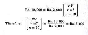
Thus an investment project of Rs. 10,000 which gen­erates an annual net cash flow of Rs. 2,000 is pro­portional to an investment of Rs. 5 that yields Rs. 1 per year. From Table A we see that at n = 10, the closest number to the present value or discount fac­tor of 5,000 is an interest rate of 15%. Therefore, this 15% interest is a close approximation to the rate of return on this investment.

(b) If management requires a minimum return of 10% on capital, this investment would surely be jus­tified since its rate of return is 5% higher than the minimum acceptable rate. In the literature on capi­tal budgeting this minimum acceptable rate of re­turn goes by the name cost of capital.

(c) From Table A (appendix) we see that at a rate of return (or cost of capital) of 10%, the present value factor for n = 10 is 6.145. Hence 6.145 x Rs. 2,000 = Rs. 12,290 is the present value of the dis­counted net cash flow.

The net present value (NPV) of investment is, then, Rs. 12,290 – Rs. 2,290; and the present value per rupee of investment, known as the profitability index or benefit-cost ratio, is Rs. 12,290 + Rs. 10,000 = 12.9%.

The profitability index is often made use of for screening proposals and for ranking investments that require identical cash outlays. However, the index must be used with care in case of investments of differing magnitudes as shown in Table 22.2.

Thus it is clear that these projects can be ranked correctly if the only criterion is the amount re­turned per rupee of investment. However, if the firm can raise sufficient capital to undertake pro­ject C, or even project D, the overall benefit to the firm will be much greater even though the profita­bility index is less. Project C, for instance, will yield more though its profitability index is less (by 8%).

The above procedure used to calculate the yield on an investment in capital goods is known as the discounted cash flow (DCF) method. This is per­haps the only method that produces the correct re­sult.

According to this method, the rate of return on an investment is “that interest rate which equates the present value of cash receipts expected to flow from the investment over its life time, with the present value of all expenditures relating to the in­vestment”.

Assume, for the sake of simplicity, that the in­vestment involves only an initial cash outlay. If it involves additional outlay in future, these, howev­er, are discounted back to the present and added to the original outlay to determine the total present value of outlays.

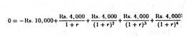
Thus, the total cost of the invest­ment may be expressed as:

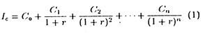
where C₀ is the initial cash outlay, C₁, C₂,… C_n are a series of future outlays, I_c the sum of all outlays properly discounted to represent the present value of the investment, and r is the market rate of inter­est which acts as the discount factor. The project will also generate a series of cash flows over its effective life that must be similarly discounted back to the present. Thus:

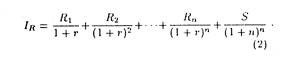
where R₁…R₂… R_n are a series of cash flows re­ceived at the end of the respective periods over the productive life of the investment, S is the scrap value at the end of n years, and I_R is the present value of this stream of future receipts.

Equation (1) expresses the present value of the investment in terms of cash outlay made. Equation (2) expresses the value of investment in terms of the cash flow generated by it.

If we succeed in se­lecting, through trial and error, that rate of dis­count r that just equates l_c to I_r, then r is defined as the rate of return on the investment. Now by setting equation (1) equal to equation (2), we arrive at equation (3) which is the most common expression for the internal rate of return (IRR) approach to capital budgeting:

 

 

 

So the internal rate of return methods involves the calculation of the rate of interest that will equate the present value of the cash outlays for an investment to the present value of the net cash flows generated by the project.

With forecasts of net cash flows for each year, it is possible to solve the above equation for the value of r such that the equality holds. This derived value of r is referred to as the IRR or yield of the investment.

From equation (3) it is clear that the IRR meth­od has two important attributes. Firstly, unlike the payback period method it considers the entire stream of cash flows generated by a project. Second­ly, whereas the ROI method and the payback peri­od method, give equal weight to future cash flows, the IRR discounts future cash flows, with the dis­count factor being the calculated IRR, denoted here as r.

Example 2:

Suppose we have the following information re­garding two investments A and B. Which project would be preferred and why?

Solution:

We may first calculate IRR of project A, i.e., the rate of interest that makes NPV of project A zero.

On the basis of the above data we have the follow­ing equation:

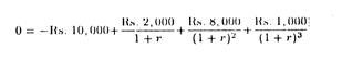
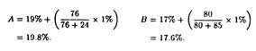
Now we can solve for r by using the trial and er­ror method. Starting from an arbitrary chosen value for r, if the right hand side of the equation is great­er (less) than zero, then a larger (smaller) value of r must be tried. If, for instance, one starts with an interest rate of 3%, the R.H.S. equals Rs. 397.60.

Therefore, we must use a higher rate of interest. If we choose 4% rate of interest, the right hand side equals Rs. 208.50. Therefore, a still higher rate must be tried. After several attempts, we will ar­rive at 5.1 rate of interest which makes the R.H.S. of the equation zero. So, according to our definition, this is the IRR for this investment.

For project B, the IRR can be determined from the following equation:

Again by following the trial and error method we find that r = 22% in this case. Therefore, project B would be preferred to (i.e., ranked higher than) project A since the former’s rate of return is larger.

The firm may now specify some minimum or accept­able rate of return, i.e., the cost of capital, which is necessary for any project to be undertaken and it will invest only in those projects whose IRR exceeds the cost of capital or the market rate of interest.

Finally, if we let e be the firm’s cost of capital and use it to discount the cash flows, we have where NPV is the net present value of an invest­ment and is used in the capital budgeting process. However, there are fundamental differences in the two approaches, viz., the IRR approach and the NPV approach. These points will be discussed in details in due course.

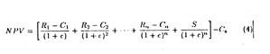
According to the NPV method any investment whose NPV (i.e., the present value of net cash flows) is positive is acceptable. The firm can rank various investment projects in order of their NPVs. Therefore, projects with the largest NPVs are ranked highest in priority, although any invest­ment with a positive NPV will add to the value (profitability) of the firm.

To illustrate how NPV is calculated and how this method is used for project evaluation we may go back to the previous example. Consider the two projects A and B assuming that the firm’s cost of capital is 10%.

For project A we have the following information:

 

 

 

 

 

 

 

 

 

 

 

 

 

It is obvious that project B will be undertaken be­cause its NPV is positive. In fact, the firm could spend Rs. 2678 more on the project without dimi­nishing the value (profitability) of the firm. On the other hand, project A cannot be undertaken be­cause it will reduce the profitability of the firm. The firm in this case would have to be paid an ini­tial sum of, at least, Rs. 819 to enable it to consider undertaking project A.

Conflict between NPV and IRR Methods:

However, there can be a conflict between the two methods because of implicit assumptions with respect to reinvestment of cash flows. The NPV method is based on the assumption that all cash inflows are reinvested at a rate equal to the cost of capital (or whatever discount rate is chosen as the cut-off rate).

Hence, all projects are evaluated against the same assumed rate of invest­ment. On the contrary, the IRR method assumes that cash inflows are reinvested at the IRR for the project. This implies that different projects have different assumed rates of reinvestment.

This may lead to conflicting conclusions with respect to the ranking of investment, as illustrated in the table below:

In Table 22.3 we consider two mutually exclusive projects to be ranked in order of desirability (e.g., setting up a flour mill or textile mill on the same plot of land). Both the projects involve the same initial cash outlay. But magnitude and timing of cash flows differ. Since they are mutually exclu­sive, only one can be undertaken.

If we evaluate both the projects by the NPV method, all net cash flows are discounted by the same 15% cost of capital and it is implicitly as­sumed that all cash flows can be reinvested to yield 15% return. However, project B having a larger NPV is preferable to project A.

Alternatively, if the IRR method is used to evaluate both the projects, we arrive at an oppo­site conclusion. Project A having an IRR of 25% is preferable to project B having an IRR of 22%. But this is because of the implicit assumption that cash flows from project A will be reinvested at 25% whereas cash flows from project B can be reinvested at only 22%.

However, in reality there is no reason why Rs. 8500 received from project A in year 2 would bring 25% in another investment while the Rs. 5000 received from project B in the same year would yield only 22%. Therefore the conclusion is that ranking by the rate of return appears to be er­roneous in this case.

However, the choice between the two methods depends upon the appropriate rate of reinvestment for the cash flows. The NPV method is considered to be superior inasmuch as all projects under consid­eration are rated against the same assumed rate of reinvestment, i.e., the common cost of capital.

iv. Rate of Return and Decision Making:

The rate of return on investment, defined by equations (1) and (2) above, goes by the name, margi­nal efficiency of capital or internal rate of return. These two concepts are identical only for a uniform series of cash flows. However, it is very difficult to apply these concepts in practice because the solution for r depends on both the amounts and the timings of the cash flows, both of which are estimates.

Thus, the rate of return is just an estimate and it would be unrealistic to insist on a precise solution for r. As Seo and Winger have commented, “the rate of return on an investment can never be stated with precision until the ownership of the investment has been terminated.”

In order to make the correct capital budgeting decision two measures are required, viz., the inter­nal rate of return and the firm’s cost of capital on the project.

Given these two choice indicators, prof­it maximization requires adherence to the follow­ing fundamental principle of marginal analysis:

Fundamental Principle:

All projects whose estimated rates of return ex­ceeds the cost of capital should be undertaken. New investment will cease when the internal rate of re­turn (or marginal efficiency of capital) equals the cost of capital.

In project selection the practical approach is to set r equal to the firm’s cost of capital. Hence the sum of the cash flows from alternative projects can be discounted by the value of r.

Then only it is pos­sible to rank projects according to their present value per rupee of investment. As a further step some doses of realism can be incorporated in the ranking process by ‘weighting’ each project by a risk factor that reflects the probability of realizing the esti­mated return.

Ranking of Capital Investments:

The essence of the capital budgeting theory is that the firm should raise the necessary capital for all non-conflicting projects that promise to in­crease the valuation of the company and thus rais­es its share prices. But in reality a firm cannot or should not raise enough capital for all of the in­vestment opportunities it faces.

There are two rea­sons for this:

(a) Projects may be mutually exclusive.

(b) There may be capital rationing problems.

In each situation the problem faced by the decision maker is how to rank investment proposals in such a way that the available capital is fully utilized in the most profitable manner.

Before discussing the above two problems con­nected with capital budgeting we may first de­scribe the relationship between the two variants of the DCF method, viz., the NPV method and the IRR method.

In Fig. 22.5 we evaluate an investment proposal that will cost Rs. 23,000 and generate annual net cash flow of Rs. 6,000 for ten years. The NPV line shows the NPV or the investment at various dis­count rates. Suppose for the sake of simplicity we ignore the time value of money. Therefore, the project will return Rs. 60,000 – Rs. 23,000 = Rs. 37,000. So the intercept on the y-axis shows Rs. 37,000.

The NVP curve slopes downward and to the right. This implies that NPV decreases with eve­ry increase in the discount rate. The IRR, it may be recalled, is that rate of discount which makes NPV zero. Here it is measured as the intercept of the x- axis where the NPV line meets it.

Here the IRR is 22.7%. So according to our fundamental principle the area under the NPV line and above the x-axis, where the cost of capital (discount rate) is less than or equal to the IRR, and the corresponding NPV is equal to or greater than zero; is the zone of acceptance.

On the contrary, the area under the NPV line and below the x-axis, where the cost of capital (discount rate) is greater than the IRR, and the corresponding NPV is therefore negative, is the zone of rejection.

v. Capital Rationing Problems:

We have noted that two discounted cash-flow methods — NPV and IRR — will always give the same accept/reject decision. It is because investment projects with an IRR in excess of the company’s cost of capital will also have a positive NPV at a rate of discount equal to the cost of capital.

Complica­tions can and do arise when the total funds availa­ble for reinvestment in a period are restricted to a fixed sum, because of management’s policy to limit investment spending, because of difficulties in rais­ing extra finance from the capital market, or for any other reason.

In such a situation managers must choose between competing projects, accepting some and rejecting others so as to stay with the compa­ny’s total funds limit. Thus the application of DCF method can prove to be problematic. In fact, when there is some limit placed upon capital expenditure so that a number of alternative proposals must be ranked in order of desirability, the NPV and IRR methods can give contradictory results.

The following example will clarify this point. Suppose a company is faced with a choice between two mutually exclusive projects, A and B, for each of which the cost of capital is the same, viz., Rs. 5,200.

The following figures show the income-flows from the projects along with NPVs and IRRs (which have been calculated for the purpose of compari­son).

Here the rate of return for project A and B are:

 

 

 

This problem is similar to the one discussed ear­lier. Both projects would be profitable to the com­pany if undertaken and would thus raise the value of the company. So it would be worthwhile for the company to borrow money at 10% to undertake both the projects.

However, a close scrutiny reveals that the rankings generated by the two DCF methods give contradictory results. If the NPV method is used, project b would be preferred to A since B has the larger positive NPV. On the contrary, if the IRR method is used, project A would be preferred to b since A has a higher rate of return.

So there is contradiction between NPV and IRR methods because of different approaches adopted by the two methods of project evaluation. The con­tradiction is also due to differences in the rate of return required by the company on investment under the two methods.

Recall that according to the IRR method, the IRR is the maximum interest that could be paid for the capital employed over its ef­fective life without any loss on the investment. If IRR exceeds the market rate of interest, the net re­turn from the investment is positive.

On the contrary, the NPV method “introduces directly into the computation the company’s mini­mum required rate of return, discounting at this rate all cash outflows and inflows form a project, down to a present value.”

The difference between the two approaches is shown clearly in the above diagram which shows NPVs for the two projects at different rates of in­terest. The IRRs of the two projects are shown by the points where the NPV schedules intersect the horizontal axis. It may be recalled that the NPV method merely shows the rates of discount which will reduce the NPVs of the two projects to zero.

On the other hand, the NPV method introduces the concept of required rate of return and NPVs can be read from the vertical axis for any chosen rate of discount. In our example the rate of discount is 10%.

Now the crucial factor in evaluating the two projects is the appropriate rate of discount to be ap­plied, i.e., the minimum acceptable rate of return on the investment. If the minimum acceptable rate of return is greater than 13% then project A would be preferred on the basis of the NPVs shown; if it is less than 13% project B would be preferred.

Thus this 13% rate is the cut-off rate, the dividing line between the two projects. The minimum acceptable rate of return may be equal to the cost of capital to a company where it is making simple accept/reject decisions.

However, as Lowes and Sparkes have argued, “where capital is rationed so that projects must compete for the limited supply of finance available, then the company must consider the op­portunity cost of capital in setting a required return. This involves considering the return on alternative projects available, and the return which might be earned investing the funds outside the firm.”

vi. Project Size and Project Life:

In reality projects do differ not only in size but also in their effective lives. These two factors add to the difficulties of comparing proposals in a capi­tal-rationing situation.

Suppose two projects differ in size. In this case the larger one having a larger NPV cannot be accepted on the ground that it is more desirable. It is because the NPV merely gives a single-figure surplus for the project and fails to relate this to the size of the investment.

The larger project may be preferred only if its NPV is propor­tionately larger than that of the smaller project. In such a situation a comparison of relative worth in­volves relating the NPVs each project to the amount of capital required by each, and then mak­ing a comparison of the ratios obtained.

If the smaller of the two projects has a higher IRR or a larger NPV then it will, of course, be pre­ferred. But it cannot be accepted on the ground that it may not represent the most profitable choice. Consider, for example, a situation where a firm has only Rs. 10,000 to invest. Suppose it is considering two projects. The first project lasts only one year. The cost of the project is Rs. 10,000.

It promises to return Rs. 11,700. So the rate of return is 17%. Sup­pose another project whose cost is Rs. 5,000 but whose life is the same promises to pay back Rs. 1,000. In this the rate of return is 20%. Thus if the company has to invest Rs. 10,000 in its entirety the second project cannot be the most profitable choice. If the company undertakes the second project it will be left with a surplus of Rs. 5,000.

If this sur­plus can earn 14%, i.e., ((7000/5000) x 100) in the company, but must be left in the bank or invested outside the company at a lower return, then it will be worthwhile to accept the larger project. It is be­cause the larger project generates a larger total sur­plus from the limited funds available to the com­pany (even if its rate of return is low).

The same type of problem crops up where pro­jects have different lives. Suppose project X costs Rs. 10,000, lasts for two years and promises a rate of return of 17%, while project Y costs Rs. 10,000, lasts three years and promises a rate of return of 15%.

Now the project profiles are presented below:

Project Y promises a larger surplus than project X. Therefore, if and only if it is possible to earn a return of at least 11.1% (i.e., ((5208.7 – 3689)/136,890) x 100) on the funds from the first project in year 3, will X be preferable.

This problem can be tackled by taking the low­est common multiple of the lives of the competing projects and comparing them over this period. In our example the period of comparison is 2 x 3 = 6 years. During this period project X would be placed only once — at the end of the third year. Total re­turns from each project can then be compared over the entire period (i.e., six years).

However, the problem here is that if we have several projects with long lives, the common multiple may be a very long period indeed. For example, three pro­jects with 8, 9 and 10 years would have to be com­pared over a 80-year period. This makes the above solution quite unrealistic.

vii. Financing Investment:

Since the profitability of a project is influenced by the cost and availability of finance from inter­nal and external sources, it is necessary to measure the cost of capital. In fact, the cost of capital de­pends on the method of financing investment pro­jects and does vary from period to period. There are various alternative methods of financing an in­vestment project.

The most important methods are the following:

(a) Earnings Plough-back:

The major portion of corporate investment in all free enterprise econo­mies is financed out of funds which are acquired in­ternally. That is, rather than distributing a major portion of company profits to the shareholders in the form of dividends, they are ploughed back into the firm for expansion and diversification.

This method offers the following advantages:

1. It avoids the heavy transactions cost asso­ciated with external borrowing or issuing new se­curities.

2. It incurs less uncertainty for management which can be sure of any funds it holds back. It can­not be very confident that its new issues of bonds and shares will evoke good public response.

3. Finally, most shareholders prefer this meth­od of financing because it converts income into capi­tal gains by increasing the market value of the company’s shares rather than providing dividend payments. This may confer substantial tax advan­tage to shareholders in the upper income brackets.

(b) Issue of New Shares or Stocks:

A company can also obtain funds through the sale of new shares. The shareholders are the actual owners of the company and they get dividends on the basis of the actual performance of the company. Thus shar­eholders are exposed to some degree of risk. A shareholder can get back his money by selling shares and make capital gains if share prices go up in a year of good business.

However, shareholders being the actual owners of the company, do take part in management. So for those companies which do not like outside control over its day-to-day operations, issue of new shares does not appear to be an attractive method of fi­nancing investment.

(c) Sale of Bonds:

Companies may borrow di­rectly from the public by selling bonds. The bond­holder gets a fixed return (interest) per annum irre­spective of the performance of the company. So bond financing may raise the fixed cost of doing business.

However, “the use of bond financing offers a distinct tax advantage since interest payments to bondholders are legally considered to be costs and are therefore not subject to the corporate income tax, whereas dividends,……….. , are considered to con­stitute income for the company and are therefore taxable.”

(d) Convertible Securities, Direct Loans, etc.:

Firms may also borrow from banks, terms-lending institutions or insurance companies. They may also issue hybrid convertibles (index bonds). The object is to protect the bondholder from the effects of price inflation (which reduces the real value of bonds).

Such bonds can be converted into shares at a specified rate of exchange such as 5: 2 or 4: 1. A convertible bond is safer than ordinary bonds and more flexible than bonds and shares inasmuch as the holder of such hybrid securities can, when he (she) sells it, dispose it of either as a bond or as a corresponding number of stocks, whichever happens to have the maximum market value at that time.

The advantage of this method of financing is that it is used by those companies which wish to pro­vide “a somewhat safer type of security or that be­lieve that the true value of its stock is not yet real­ized by the market. When the price of the company’s stock rises sufficiently, the holder of convertibles will all find it profitable to transform them into stocks, and this will then automatically eliminate any bonded company indebtedness which the securities originally represented.”

Now we speak of cost capital on the basis of the above discussion.

The Cost of Capital:

The cost of capital establishes a standard that enables management to divide prospective projects into two broad groups: those that are acceptable and those that are not. Moreover, the cost of capi­tal together with rates of return on available pro­jects determines the optimum amount of total invest­ment that should be made during the planning period of the business firm.

The economic concepts of demand and supply may now be fruitfully utilized to throw light on the capital budgeting process which is basically an aspect of financial management.

If different investment proposals are ranked in order of their estimated rates of return, along with the respective capital outlays on them, one can con­struct the firm’s demand schedule for capital. Then the problem would be simply to determine a supply schedule of capital.

The interaction of the two schedules would determine the desired volume of investment of a profit-maximising firm. In Fig. 22.7, the cost of capital is 12%. So all projects which promise a return in excess of this initial rate would be accepted; similarly those projects whose estimated rates are less than this critical rate would be rejected.

In Fig. 22.7 the firm has 8 differ­ent proposals — starting from A and ending up with H — for consideration during the current planning period. The first project promises a return of 25% which is highest here and it requires as initial out­lay of Rs. 2 lakhs. Project H promises the lowest re­turn (7%) and involves an outlay of Rs. 4 lakhs.

The rates of return of all other projects lie in-between these two extremes. The MCC line is the firm’s sup­ply curve of capital. It shows the marginal cost of capital to the firm in respect of both internal and external finance.

The curve is completely elastic up to a certain level of investment e.g., Rs. 25 lakhs. After this it slopes upward and to the right. This implies that the cost of capital will increase more than proportionately after a certain stage.

Such a situation may be due to two factors:

1. The external capital market may become im­perfect in a period of business expansion when all firms increase their expenditure on plant and equipment.

2. The inability of the firm to utilize capital be­yond a particular point without substantially altering the risk exposure of shareholders or creditors.

It is clear from Fig 22.7 that only the first five projects should be undertaken since their rates of return exceed the marginal cost of capital. This would involve a total expenditure of Rs. 11.5 lakhs.

By the term ‘cost of capital’ which is an essen­tial criterion for investment decision making, we refer to the marginal cost of capital, i.e., the extra cost of acquiring an extra unit of capital to be uti­lized by the firm during the planning period.

Since the firm has alternative sources of finance, the most commonly used method is to calculate the weighted average of the current cost of funds of the firm from all sources. This amounts to calculating the cost of debt and the cost of equity which are the two major sources of business finance.

However, an important point has to be clarified at the outset. The cost of debt is partly influenced by the cost of equity inasmuch as to be able to en­gage in debt financing (that is, selling bonds or bor­rowing from financial institutions), a company must have an adequate equity case.

This is why an ap­propriate debt equity norm has been set for the In­dian corporate sector. In every country there is a le­gal provision in this matter. If a firm incurs a debt, it is under the legal obligation to make periodic in­terest payments before its earnings can be distribut­ed to its owners in the form of dividends. Therefore the existence of an equity base proves that its cred­itors are safe.

It may be noted that the greater the proportion of total assets that are financed by debt as com­pared to equity, the greater the potential financial loss to the equity-holders (the owners), in a year, of bad business (when earnings decline). It is because after paying fixed interest the company may not be left with any surplus for distribution as dividends.

So dividends have to be skipped for a year or two in succession. On the contrary, if the firm can earn more on its total assets than the fixed interest that it pays to the bondholders (its creditors), the shar­eholders will receive higher dividend earnings. This is known as ‘trading on the equity’, or ‘lever­age’ in financial management.

Calculating the Cost of Capital:

From the above discussion one can guess that an ‘optimum’ or ‘best’ financial structure exists for eve­ry firm, or at least within which the debt/equity ratio is ideal under the present circumstances. Therefore, when a firm incurs additional debt fi­nancing, it uses up some of its existing equity base. If this continues, the financial structure of the compa­ny will be unbalanced in favour of debt.

We may note that the cost of capital is actually weighted average of the current cost of funds from all possible sources. An estimate of such cost is based on market costs of debt and equity (rather than historical costs or book values) because invest­ment decisions are made on the basis of current (rather than past) information. Table 22.4 illus­trates how the weighted cost of capital is calculat­ed.

It was pointed out that the cost of debt is a de­ductible expense for income tax purposes, but the cost of equity is not. Here the cost of capital is 12.7% which is the minimum that must be earned on the total cash outlay on a project. To this, man­agement may add a safety margin.

Each method of financing has two sides: First­ly, it generates net revenue for the firm (after in­curring all transaction costs). Secondly, it involves some future cash outflows, such as interest pay­ments, repayment of principal or payment of divi­dends.

The rare of discount which equates the present value of net cash inflows with the present value of the expected outflows is the explicit cost of the particular source of financing involved and is calculated by using the following equation:

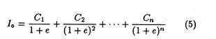
where I₀ is the net income, or yield, of the method of financing; C_i is the cash outflow in the period i = 1,2, n, and e is the rate of discount that express­es cost (before tax) of the method of financing. This formula may be used for making the cost estimate for each specific source of capital.

Cost of Debt:

We have noted in Table 22.4 that the average cost of capital to a firm in any given year is a weighted average cost of the percentage annual cost of equity (funds obtained by retaining earnings or by selling additional shares). Now we may examine the cost of debt and the cost of equity separately.

The before-tax cost of debt is the nominal inter­est rate. If a firm has both short-term and long- term debt at differing interest rates, after-tax cost of debt is the weighted average of these rates. Af­ter-tax cost of debt is reduced because interest pay­ments are deductible expenses for tax purposes.

Cost of Equity:

Equity capital consists of funds obtained from the sale of common stock plus the retained earnings of the firm. The market price of an equity is based upon the expectations and attitudes of investors to­ward risk. Thus the cost of equity is the minimum rate of return that will keep the market price of the stock unchanged.

It is simply the present value of the expected future income stream from the equi­ty and can be expressed as:

where D₁, D₂,………. D_n are a series of cash dividends received at the end of each of the respective peri­ods over the life of the investment; S_n is the market value at the end of n periods; e is the investor’s re­quired rate of return (the discount factor); and I is the present value of the investment.

If the company’s dividends are expected to grow at a constant (steady) rate for ever, then the divi­dends in any period may be closely approximated with the most recent dividend multiplied by the compound growth factor.

On the basis of this as­sumption we can arrive at an alternative expres­sion:

C_e = D₁/P₀ +g

where the cost of equity C_e is the ratio of the next expected dividend D₁ to the current price P₀ plus the rate of growth, g. This equation can be used to de­rive the cost of capital, provided that both the timing and the magnitude of changes in the growth pattern can be estimated.

Thus if the current price of an equity share is Rs. 50, the current dividend is Rs. 3 per share, and projected rate of gain in earning per share and share price is 8% per annum, the cost of equity is

Rs.3/Rs. 50 + 0.08 = 0.14 or, 14%

viii. The Certainty-Equivalent Method:

A number of techniques is available for express­ing IRR or NPV on a risk-adjusted basis. However, the most popular method is the certainty equival­ent method (CEM), discussed in a preceding chap­ter.

The CEM starts by assessing the risk character­istics of each project’s annual cash flows and subse­quently reduces the cash flows to certainty- equivalent amounts. Fig. 22.8 shows how this is achieved on the basis of the decision-makers will­ingness to trade off risk and return.

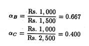
In Fig. 22.8 the decision-maker is assumed to have three invest­ment choices : A, B and C. Project A has zero risk and offers a moderate return of only Rs. 1,000; project B and C are more risky and therefore offer higher re­turns (e.g., Rs. 1500 and Rs. 2500, respectively).

Their risks are measured by coefficients of varia­tion vB and vC, respectively. The locus of these three points can be thought of as the decision-makers risk-return indifference curve.

Therefore, the decision maker is indifferent among all the three pro­jects and hence cannot rank them in order of prefer­ence. In short, these are risk-adjusted equivalent- yield investments, where the added returns at­tached to B and C are totally offset by the greater risk which is associated with them.

For projects B and C, certainty equivalent weighted factors (a-values) are determined from Fig. 22.8 as follows:

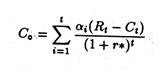
These a-values may now be used in the follow­ing formula that yields r*, the certainty equivalent IRR for the ith project:

Alternatively we can make use of a-values to determine the certainty equivalent NPV denoted as NPV’:

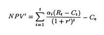
where r’ is the rate of return on a-risk-free invest­ment (such as a government bond) economic and t is the life of the project.

Now the decision for accepting or rejecting an investment is:

(1) Accept all project where r* > r’; or

(2) Accept all projects with positive NPV’.

It may be noted that the derived a-values are unique in the sense that they are applicable to all projects having risk characteristics of v_A and v_B. In other words, the decision maker should be consis­tent in treating risk from investments by matching α-values with v-values.

However, for practical convenience, it is better to express these values for broad categories of risk such as very high risk (a₂) high risk (a₂), medium high risk (a₃), low risk (a₄), and so forth, rather than having a wide range of a-values. This will make the process more man­ageable.

ix. Other Methods for Handling Risk:

Two other methods of handling risk in an in­vestment decision situation are:

(1) The risk- adjusted discount rate approach and

(2) A probabil­ity distribution approach.

With the first approach, the decision maker must specify at the outset the degree of risk in a particular investment decision. If the risk exceeds the risk of an ‘average’ invest­ment, a risk premium has to be added into the ‘av­erage’ discount rate. This risk-adjusted discount rate is to be used to calculate net present values. It follows quite logically that investments with less than the average risk are discounted at lower rates.

However, this approach has two major defects. Firstly, it is not possible to determine the risk- adjustment factor objectively. So, some link element is involved in its measurement as in case of deter­mination of a-values in the CEM.

Secondly, like the CEM, this method makes no allowance for peri­od to period risk adjustments. It just makes a single adjustment to the discount rate which is then ap­plied to each annual cash flow.

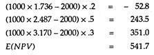
The probability distribution approach is slightly better than the previous two methods. It calculates an NPV amount for each possible outcome related to an investment. Consider, for instance, a project that costs Rs. 2000 and is expected to gener­ate a net cash flow of Rs. 1000.

The decision maker does not know with certainty for how many years this flow will continue. This can at best be ex­pressed in probabilistic terms.

Assume that these periods are possible with the following probabili­ties:

(1) two year, p = .2,

(2) three years, p = .5; and four years, p = .3.

Using a discount rate of 10% we have the following expected NPV:

Modern financial analysts and project managers calculate, in addition, a standard deviation to de­termine the degree of variation in NPV which is then used to assess the project’s risk. However, the decision maker has still to determine a risk-return trade-off function before reaching a decision. So to this extent, the probability distribution approach is equivalent to the previous two approaches.

So there are various methods of methods of in­vestment appraisal or project evaluation, each having its advantages and disadvantages. In the ultimate analysis, “the choice of a particular method should be made on the basis of operational simplicity and ease of understanding, rather on the basis of strong theoretical arguments.”

---

7. Capital Budgeting under Risk and Uncertainty:

So long we assumed that there is complete cer­tainty in the investment selection decision. But this assumption is unrealistic inasmuch as invest­ment projects last for many years and the future can hardly be predicted with certainty. There are two major sources of uncertainty in any capital budget­ing process.

Firstly, in case of most projects, the es­timated annual cash flow represents the expected value of a weighted probability distribution of ac­tual cash flows, i.e., each cash flow is weighted by an appropriate probability estimate.

In fact, in most practical situations, some cash flows may be the product of joint probability distributions for both cash inflows and outflows. Secondly, the life of a project is also uncertain in most cases. So we have to take note of these realities and adjust them for their relative risks.

---