Fiscal and Monetary Policy Change (With Diagram)

It may be noted that the fiscal policy change (a change in taxes or government expendi­tures) will shift the IS curve, and monetary policy change will shift the LM curve.

a. Monetary Policy:

Monetary policy attempts to stabilise the aggregate demand in the economy by regulating the money supply. An expansionary monetary policy is needed to stimulate the economy.

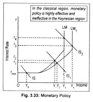
This makes the LM curve to shift to the rightward direction. Note that in Fig. 3.33, we have drawn negative sloping IS curve and positive sloping LM curve.

The LM curve has three stages:

(i) Liquidity trap region where the LM curve is horizontal (also known as the Keynesian region),

(ii) The classical region where the LM curve is vertical, or perfectly inelastic, and

(iii) The intermediate region where the LM curve is positively sloped.

In the liquidity trap region or extreme Keynesian range, monetary policy is totally ineffective in stimulating income. Despite an increase in money supply, LM curve does not change its position. An increase in money supply cannot cause the interest rate to fall below the rate given by the liquidity trap. Equilibrium income then remains unchanged at OY₀.

As was believed by Keynes during the Great Depression years of the 1930s that the economy was caught in the trap region then he recommanded for the use of unorthodox fiscal policy. In other words, monetary policy was to be discarded during the early 1930s as it would be grossly ineffective instimulating the economy.

The essence of the argument is that since government is helpless in raising income/output level through monetary policy, the government has to employ the fiscal policy. Anyway, it must be said that the liquidity trap is an extreme case.

Secondly, in the classical region, where the LM curve is vertical, monetary policy becomes completely effective. As the LM curve shifts to LM₁, rate of interest declines more this time from Or₄ to Or₃. This causes income to rise by a larger amount from OY₃ to OY₄. In view of this, classicists favour monetary policy.

But Keynesians reject monetary policy during depression when rate of interest reaches a floor level. Thus, in the classical range, monetary policy is completely effective in contrast to the Keynesion or liquidity trap region in which monetary policy is totally ineffective, (i.e., the LM curve is perfectly elastic).

Finally, in the intermediate range where the LM curve is positive sloping, an increase in money supply shifts the LM curve from LM to LM₁. Consequently, interest rate declines to Or₁ and income rises from OY₁ to OY₂. Thus, monetary policy is effective. To be more specific, monetary policy is found to have a degree of effectiveness but not the complete effectiveness as we see in the classical region.

In general, the closer the equilibrium (of IS and LM curves) is to the classical region, the more effective monetary policy becomes, and the closer the equilibrium is to the Keynesian range, the less effective monetary policy becomes.

b. Fiscal Policy:

Fiscal policy also attempts to influence aggregate demand in an economy by influencing tax-expenditure programme of the government. A cut in taxes or an increase in government spending causes a shift in the IS curve in the rightward direction.

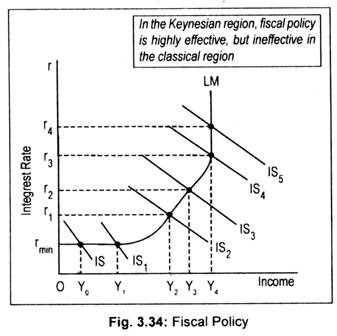
In Fig. 3.34, the IS curve intersects the LM curve at its horizontal portion (i.e., liquidity trap region). In this region, as the IS curve shifts from IS to IS₁, the equilibrium level of income rises from OY₀ to OY₁. Thus, fiscal policy is completely effective in stimulating aggregate income in the depressionary phase without having any effect on interest rate.

Secondly, in the classical range, fiscal policy is completely ineffective since it fails to stimu­late aggregate demand and, hence, aggregate income. Fig. 3.34 says that the increased gov­ernment expenditure and/or decreased taxes shifts the IS curve in the classical region (where the LM curve is vertical) from IS₄ to IS₅. This causes equilibrium intersection to shift up. This results in an increase in the interest rate only from Or₃ to Or₄, keeping income level unchanged at OY₄.

Finally; fiscal policy is partly effective in the normal intermediate range where both interest rate and income rise. Fiscal measures that shift the IS curve from IS₂ to IS₃ in the section between Keynesian and classical section, called, intermediate section, raises the level of income from OY₂ to OY₁ and the rate of interest from Or₁ to Or₂.

Thus, fiscal policy is found to have a degree of effectiveness in this region. It may be concluded that in general fiscal policy becomes more effective the closer the IS-LM intersection or equilibrium lines to the Keynesian or liquidity trap region and less effective the closer equilibrium resides to the classical region.

Thus, fiscal policy may be employed in depression years. This is the Keynesian argu­ment. It is argued that these results concern­ing monetary policy are the opposites of the results obtained under fiscal policy regime.

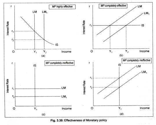
Thus, one can conclude that the effective­ness of monetary policy depends on (i) the interest-elasticity of the demand for money, and (ii) the interest elasticity of investment. These two aspects can be illustrated in terms of Fig 3.35.

If the LM curve is vertical (pure classical case), monetary policy becomes highly effective in raising equilibrium income [Fig. 3.35(a)]. Consequent upon an increase in money supply, the LM curve shifts from LM to LM₁. Equilibrium interest rate now declines from Or₁ to Or₂ and equilibrium income rises from OY₁ to OY₂.The biggest effect of monetary policy can be felt if the IS curve is perfectly elastic [Fig. 3.35(b)]. Note that following a shift in the LM curve from LM to LM₁ national income rises from OY₁ to OY₂ without influencing the interest rate that remains at Or₁.

On the other hand, if the LM curve is horizontal (pure Keynesian range) and if the IS curve is vertical, monetary policy becomes ineffective completely [Figs. 3.35 (c) and (d)]. Fig. 3.35 (c) says that a downward shift in the horizontal LM curve from LM to LM₁ along with the vertical IS curve, income remains unchanged at OY₁ while r declines to Or₂.

Thus, monetary policy does not have any influence in stimulating an economy in depression. Again, monetary policy fails to boost income/output of an economy if the positive sloping LM curve shifts from LM to LM₁, though interest rate declines from Or₁ to Or₂ following an increase in money supply.

Likewise, the effectiveness of fiscal policy depends on the slopes of the IS curve and the LM curve. The more interest-inelastic is the investment, the more effective is fiscal policy (Fig. 3.36(b). Likewise, the flatter the LM curve, greater the effectiveness of fiscal policy (Fig. 3.36 (c). Fiscal policy is completely in­effective in Fig. 3.36(a).