The article mentioned below provides an algebraic analysis of IS-LM model.
The Derivation of IS Curve: Algebraic Method:
The IS curve is derived from goods market equilibrium. The IS curve shows the combinations of levels of income and interest at which goods market is in equilibrium, that is, at which aggregate demand equals income.
Aggregate demand consists of consumption demand, investment demand, government expenditure on goods and services and net exports.
Consumption demand is function of disposable income. Disposable income is level of income minus taxes (Yd = Y – T) where Yd stands for disposable income and T for taxes. However, in a two-sector model where we do not incorporate taxation by the government, Yd = Y.
ADVERTISEMENTS:
Investment depends on rate of interest. With a given level of income, a higher rate of interest reduces investment demand and a lower rate of interest leads to more investment, that is, investment is negatively related to rate of interest. Thus,
I = I – di
Therefore, we have the following equation for aggregate demand (AD)
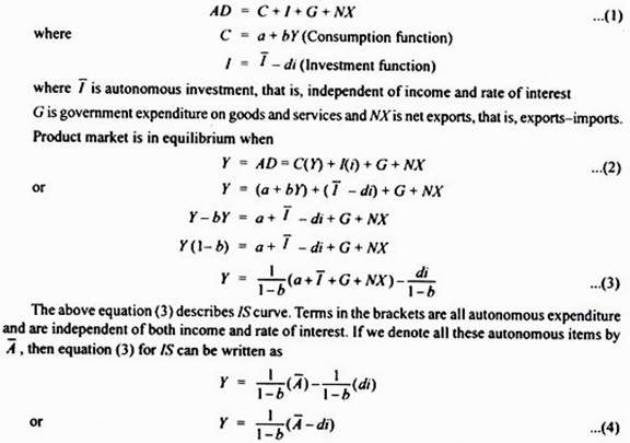
1/1-b is the income multiplier and b is marginal propensity to consume. Given the value of autonomous expenditure, we can obtain value of Y at different rates of interest to draw an IS curve. It is worth noting that the value of autonomous (A) determines the intercept of the IS curve, d in the term di in equation (3) shows the sensitivity of investment to the changes in rate of interest and determines the slope of IS curve. Since fall in interest rate increases investment spending, it will raise aggregate demand and thus the equilibrium level of income. Besides, the slope of the IS curve depends on the size of income multiplier.
ADVERTISEMENTS:
Problem 1:
The following equations describe an economy:
C = 10 + 0.5 Y (Consumption function)
ADVERTISEMENTS:
I = 190-20i (Investment function)
Derive the equations for IS curve and represent it graphically.

At 2 per cent rate of interest, level of income is 320.
We have now two combinations of interest and income. We can plot these and obtain IS curve. This is done in Figure 20.18.

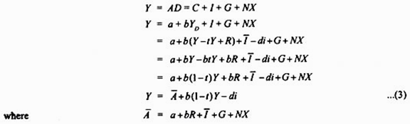
IS Curve: Three-Sector Model with Taxation and Transfer Payments:
In the last section we have derived the IS curve taking government expenditure G on goods and services without considering taxation and transfer payments by it. In fact the concept of consumption function conceives consumption as a function of disposable income and is therefore written as
C = a + bYD …(1)
Now, disposable income YD is obtained from deducting tax and adding transfer payments by the government. Thus
ADVERTISEMENTS:
YD = Y – T + R
where T is tax revenue and R is the transfer payments by the government. Whereas a tax reduces disposable income, transfer payment raises it.
Further, whereas transfer payments are assumed as lump sum amount, tax can be lump sum tax or levied as proportion of income. If we assume proportionate income tax, then,
T = tY
ADVERTISEMENTS:
where t is the proportion of income which is taken away by way of tax. …(2)
Let us derive IS equation incorporating proportionate income tax and lump sum transfer payments.
ADVERTISEMENTS:
where 1/1-b(1-t) is the value of multiplier in case of proportionate income tax. Equation (4) represents IS curve in case of proportionate income tax.
It may be noted in the context of IS equations (3) and (4) that a change in autonomous spending (A) as a result of any of its components will cause a shift in IS curve.
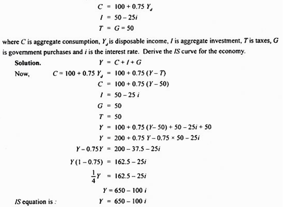
Problem 2:
The following equations describe an economy:
Derivation of LM Curve: Algebraic Analysis:
Having derived algebraically equation for IS curve we now turn to the derivation of equation for LM curve. It will be recalled that LM curve is a curve that shows combinations of interest rates and levels of income at which money market is in equilibrium, that is, at which demand for money equals supply of money.
ADVERTISEMENTS:
We explain the derivation of LM curve in two steps. First, we show how money demand depends on interest rate and level of income. It is worth noting that in their demand for money people care more about the purchasing power of money, that is, people’s demand is for real money balances rather than nominal money balances. Real money balances are given by M/P where M stands for nominal money demand and p for price level.
The demand for real money balances depends on the level of real income and interest rate. Thus Md = L(Y, i). Demand for real money balances increases with the rise in level of income and decreases with rise in rate of interest. Let us assume that money demand function is linear. Then
L(Y, i) = kY – hi k, h > 0 …(5)
Parameter k represents how much demand for real money balances increases when level of income rises. Parameter h represents Low much demand for real money balances decreases when rate of interest rises. The equilibrium in the money market is established where demand for real money balances equals supply of real money balances and is given by
M/P = kY – hi …(6)
Money supply (M) is set by the central bank of a country and we assume it to remain constant for a period. Besides, we assume the price level (P) to remain constant.
ADVERTISEMENTS:
Solving the equation (6) for interest rate we have
i = 1/h (kY – M/P) …(7)
The above equation (7) describes the equation for LM curve. To be precise it gives us the equilibrium interest rate for any given value of level of income (Y) and real money balances. In drawing LM curve, real money balances are assumed to be constant.
Thus LM curve describes money market equilibrium for different values of income and rate of interest, given a fixed value of real money balances (M/P). Thus, given the real money balances (M/P), we can obtain a rate of interest for different values of income.
Let us state some conclusions about LM curve as given by equation (7). First, since in equation (7) for LM curve, the coefficient (k) of income (Y) is positive, LM curve will slope upward. That is, higher income requires higher interest rate for money market to be in equilibrium, given the supply of real money balances.
Second, since the coefficient of real money balances is negative, the expansion in real money balances will cause a shift in the LM curve to the right, and decrease in the real money balances will shift LM curve to the left.
ADVERTISEMENTS:
From the coefficient of income k/h, we can know whether LM curve is steep or flat. If demand for money is not much sensitive to level of income, then k will be small. Therefore, in case of small k (i.e. low sensitivity of interest with respect to changes in income), small change in interest rate is required to offset a small increase in money demand caused by a given increase in income.
Problem 3:
Given the following data about the monetary sector of the economy:
Md = 0.4 Y – 80i
Ms = 1200 crores.
where Md is demand for money, Y is level of income, Ms is rate of interest and M is the supply of money
ADVERTISEMENTS:
1. Derive the equation for LM function
2. Give the economic interpretation of the LM curve. Draw LM curve from the above data
Solution:
For money market to be in equilibrium:
Md = Ms
0.4 Y – 80 i = 1200
80 i = 0.4 Y – 1200
i = (0.4Y/80) – (1200/80)
i = (1/200) Y – 15 ….. (i)
Thus we get the following LM function:
i = (1/200) Y – 15
Alternatively, LM equation or function can also be stated as:
Y = 200i + 3000 …(ii)
LM curve means what would be rate of interest when money market is in equilibrium, given the level of income. Thus, if level of national income is Rs. 4000 crores, then using LM equation (i) we have
i = (1/200) x (4000 – 15)
= 20 – 15 = 5%
Thus, at income of Rs. 4000 crores, rate of interest will be 5 per cent when money market is in equilibrium.
Now, if level of income is Rs. 4400 crores, equilibrium rate of interest will be
i = (1/200) Y – 15
= (1/200) x (4400 – 15)
= 22 – 15 = 7%
With two combinations of interest rate and income level when money market is in equilibrium we can draw LM curve as shown in 20.19.

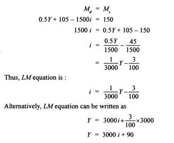
Problem 4:
The following data is given for the monetary sector of the economy:
Transaction demand for money, Mt = 0.5Y. Speculative demand for money, Msp = 105 – 1500 i
Money supply Ms = 150
Derive LM equation from the above data
Solution:
Total demand function for money can be obtained by adding up the transactions demand for money (M) and speculative demand for money (Msp). Thus
Md = Mt + Msp
Md = 0.5 Y + 105 – 1500i
In money market equilibrium
IS – LM Model: Algebraic Analysis (Joint Equilibrium of Income and Interest Rate)
The intersection of IS and LM curves determines joint equilibrium of income and interest rate. Mathematically, we can obtain the equilibrium values by using the equations of IS and LM curves derived above. Thus,

Joint determination of equilibrium values of income and interest rate requires that both the IS and LM equations hold good. In this way both the goods market and money market equilibrium will be achieved at the same interest and income levels in the two markets. To find such equilibrium values we substitute the interest rate from the LM equation (ii) into the IS equation (i). Doing so we have
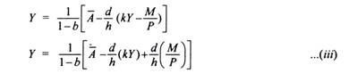
The equation shows that the equilibrium level of income depends on exogenously given autonomous variables (A) such as autonomous consumption, autonomous investment, government expenditure on goods and services, and the real money supply (M/P) and further on the size of multiplier (1/1-b). It will be noticed from equation (iii) that higher the autonomous expenditure, the higher the level of equilibrium income. Further, the greater the real money supply, the higher the level of national income.
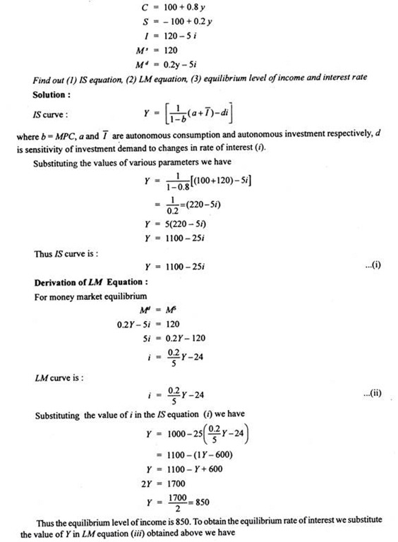
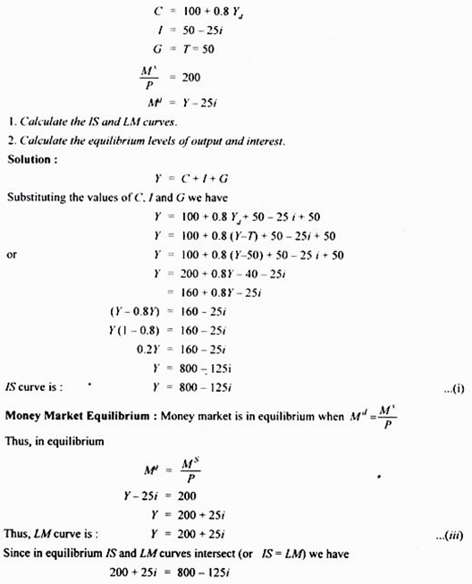
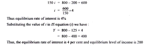
Problem 5:
For an economy the following functions are given:

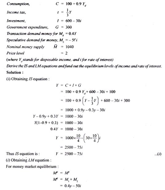
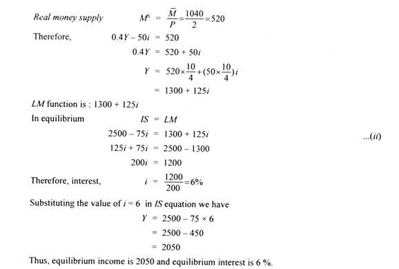
Problem 6:
Consider the following economy:
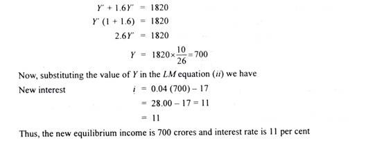
Problem 7:
Consider an economy with the following features:
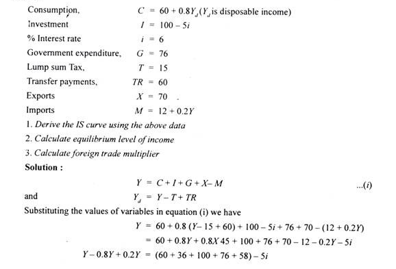
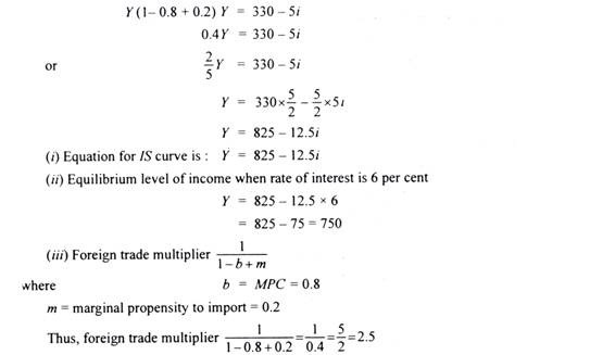
Problem 8 (Four-Sector Model):
The major macro aggregates for an economy are given as follows:
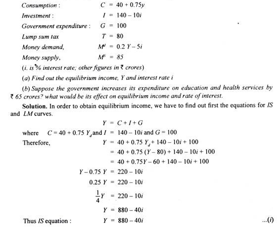
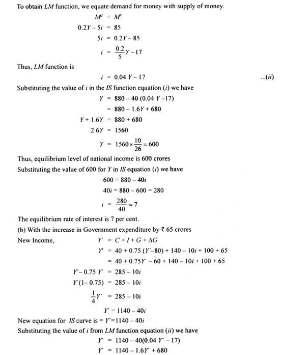
Problem 9:
The following data are given for an economy:
Problem 10: