IS-LM Curve Model: Structure, Usefulness and Limitation (With Diagram)

Let us make an in-depth study of the IS-LM Curve Model. After reading this article to learn about: 1. Structure of the IS-LM Model 2. The Basic IS-LM Curve Model 2. Usefulness 3. Limitation.

Structure of the IS-LM Model:

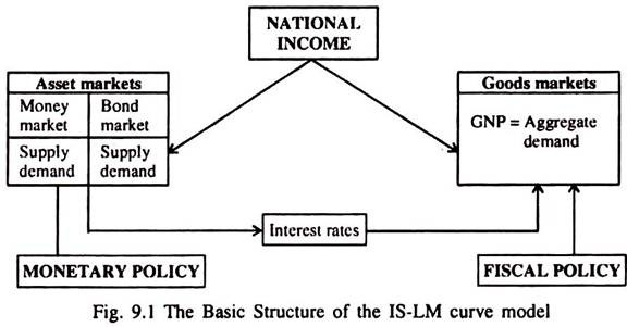
The IS-LM curve model emphasises the interaction between the goods and assets markets.

The Keynesian model looks at income determination by arguing that income affects spending, which, in turn, determines output (GNP) and income (GNI).

J. R. Hicks and A.H. Hansen add the effects of interest rates on spending, and thus income and the independence of asset markets on income.

Higher income raises money demand and thus interest rates. Higher interest rates lower spending and thus income. Spending, interest rates and income are determined jointly by equilibrium in the goods and assets markets as shown in Fig. 9.1.

.

1. Role of Money in the Simple Keynesian System:

The central proposition of Keynes’ theory of money is that money affects income via the interest rate. If money supply increases, the rate of interest falls. The lower interest rate, in its turn, leads to a rise in autonomous investment and in national income through the autonomous expenditure multiplier.

2. Interest Rates and Aggregate Demand:

Keynes pointed out that business investment demand depends on the interest rale. In his view, an investment project will be carried only if its expected rate of return (or marginal efficiency of capital) exceeds the cost of borrowing to finance the project so that the net return from the project is positive. For this reason at a higher interest rate (borrowing cost), fewer projects will be accepted.

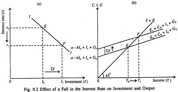
In Fig. 9.2 we show the effects of interest rate changes on aggregate demand. In part (a) a fall in the interest rate from r₀ to r, increases investment by ΔI from I₀ to I₁. This shifts the aggregate desired expenditure schedule upward – from E₀ = C₀ + I₀ + G₀ to E₁ = C₀ + I₁, + G₀ . As a result output (income) increases from Y₀ to K, in part (b).

3. The Keynesian Theory of the Interest Rate:

In Keynes’ theory the quantity of money plays a key role in interest rate determination. The demand for money (liquidity preference) is the crucial variable in Keynesian theory of money.

Keynes makes two assumptions:

(1) All financial assets can be divided into two groups, viz., money and homogeneous bonds (i.e., all non-monetary assets).

(2) Money pays no interest.

At a fixed point in time, an individual has a fixed amount of wealth (W) which is divided between money (M) and bonds (B):

W = M + B … (1)

So more money holding implies less bond holding and vice versa. Thus there is only independent portfolio decision, the division of W between M and B. Therefore, an excess demand for money implies an excess supply of bonds and an excess supply of money implies an excess demand for bonds.

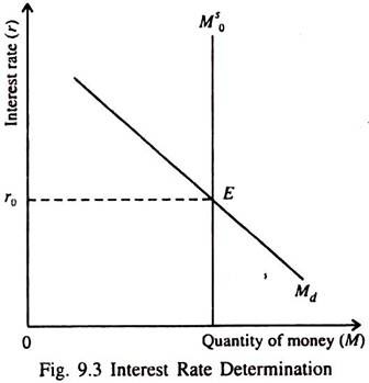
In Keynes’ model the equilibrium rate of interest (r₀) is determined by the demand for money and the supply of money as shown in Fig. 9.3.

Since the money supply is assumed to be fixed exogenously by the policy of the central bank at M₀^S, the demand for money plays the key role in determining the rate of interest. We may now discuss the factors determin­ing the position and slope of the money demand curve (M_d).

The Keynesian Theory of Demand for Money:

Keynes discussed and analysed three separate motives for holding money:

(a) Transactions demand:

Since money is a medium of exchange, people hold money for purchasing goods and services or for making any type of payments. Money bridges the time gap between the receipt of income and its expenditure. Transactions demand for money varies directly with the volume of transactions which is assumed to depend positively on the level of income.

(b) Precautionary demand:

People also hold money to meet unexpected expenditures, known as the precautionary demand for money. It also depends positively on income. Here we include the precautionary demand under transactions demand (and do not treat the former separately).

(c) Speculative demand:

Finally, people hold money for speculative purposes even if bonds pay interest and money does not. The reason for this, in Keynes’ view, is uncertainty about future interest rates and the relationship between changes in the interest rate and the price of bonds.

The price of bond is the reciprocal of the rate of interest. Thus if the market rate of interest rises (falls) the price of an old bond will fall (rise) and the bondholder will incur a capital loss (or make a capital gain).

For example, if the current market rate of interest is 5% and a bond promises to pay a fixed sum of Rs.10 per annum, its market price is:

where B is the price of bonds, A is fixed return on bonds and r is the market rate of interest. If r rises to 10% B_p will be Rs.10/10% = Rs.10/(1/10) = Rs.100. If r falls to 2½%, B_p will be Rs.10/(1/40) = Rs.400.

If an individual holds only money there is no risk and there is no return either. If he buys bonds, he earns interest but faces uncertainty. In case the rate of interest rises (falls) he will incur capital loss (make capital gains) on old bonds.

The expected return on money is zero. But the expected return on bonds has two components:

(a) Interest r plus expected capital gain or r minus expected capital loss. This uncertainty about the future course of interest rates is of crucial significance to Keynes’ analysis.

So while holding bonds an individual has to strike a balance between two conflicting things. If interest rates are expected to fall, bonds will have the higher expected return in terms of interest and capital gains. If interest rates are expected to rise, the expected capital loss on bonds will outweigh the interest earnings.

In such a situation the expected return on bonds would be negative and money would be preferred to bonds. Speculative demand for money refers to money held in anticipation of a fall in the prices of bonds (i.e., a rise in interest rates).

Keynes assumes that when the actual rate of interest goes above the normal level, investors expect it to fall. When the interest rate is below the normal level, they expect it to rise.

This relationship between the level of the speculative demand for money and the interest rate may initially be illustrated in case of an individual investor and then in the case of the market as a whole, (i.e., the corresponding aggregate relationship).

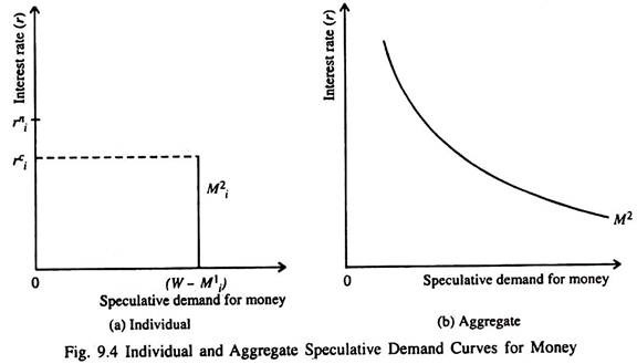
For an individual investor (i), the demand curve for speculative balances is shown in Fig. 9.4 (a).

Here we have

where M_i is total demand for money, M_i¹ is the transactions demand, M_i² is the speculative demand, B_i is bond holding and is his total wealth. At any rate of interest above the critical rate (r_i), the speculative demand for money is zero. Below it, the individual holds only money.

Part (b) shows the aggregate speculative demand for money curve (M). As the interest rate falls below the critical rate for most individuals, the speculative demand for money will increase.

This is why the speculative demand curve in Fig. 9.4 (b) is downward sloping. The smoothness of the curve indicates the gradual increase in the speculative demand for money at lower and lower rates of interest.

According to Keynes, it costs money to hold money and the market rate of interest (r) is the opportunity cost of money holding. When the rate of interest is very low most people can afford the luxury of money holding.

At the same time when the rate of interest is very low, most people — if not all, expect it to rise in future, in which case the price of bonds will fall. So to avoid possible capital losses people prefer to hold as much money as possible.

At all rates of interest above r_in in Fig. 9.4 (a), interest rates are expected to fall and bond prices expected to rise (giving a chance of making capital gain). If the interest rate does not fall much below r_in, the interest earnings on the bond will be greater than the small expected capital loss.

As r continues to rise and moves towards r_in there will capital loss but this will be less than the interest income as long as r_in < r_ic. So no money will be held and all wealth will be held in bonds.

At a very low rate of interest, all investors expect r to rise in future. So the liquidity preference curve gradually flattens out at a very low rate of interest, reflecting that at this rate, most — or even all — people expect capital losses on bonds that outweigh interest earnings.

At this rate, all existing wealth (including additions to it) are held in money. So the speculative demand curve for money becomes completely elastic at this critical rate of interest.

Any increase in the stock of money by the central bank will be absorbed by the people in the form of liquidity balances and this will prevent the rate of interest from falling further. This means that the speculative demand curve for money becomes completely elastic. The completely elastic part of the M₂ curve is known as the liquidity trap situation.

Keynes argued that in a depressed economy which is experiencing a liquidity trap, the only way to stimulate investment is to increase Government expenditure or reduce taxes in order to increase aggregate demand and improve business confidence about future prosperity, encouraging them to invest.

In short, the term ‘liquidity trap’ was used by Keynes to refer to a situation at a very low rate of interest where the speculative demand for money curve becomes almost completely elastic (nearly horizontal). This type of situation is normally observed during depression. In normal times the speculative demand curve for money is assumed to slope downward.

4. The Total Demand for Money:

Since transactions demand for money varies directly with income and speculative demand for money inversely with the rate of interest, the total demand for money is a function of both the variables and can be expressed in functional form, as

M^d = L(Y, r) … (3)

where Y is income and r is the interest rate while a rise in Y increases M^d, a rise in r reduces it, i.e., dM^d/dY > 0 and dM^d/dr < 0.

If we assume that the money demand function is linear it can be expressed in the following form:

M^d = c₀ + c1Y – C₂r, c_2r, > 0; c₂ > 0 … (4)

Here c₁ shows the increase in the demand for money per unit increase in income and c₂ is the amount by which M^d falls with every unit increase in the interest rate.

5. The Effect of an Increase in the Money Supply:

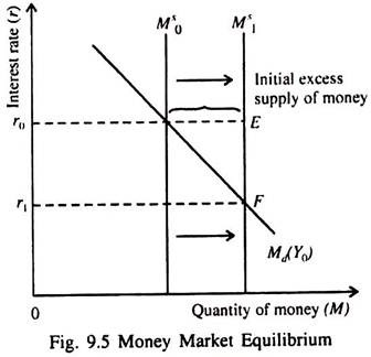
An increase in the supply of money from M₀^s to M₁^s initially creates an excess supply of money. This is equivalent to an excess demand for bonds. As a result, the price of bond rises. This is equivalent to a fall in the rate of interest. In Fig. 9.5 the rate of interest falls in from r₀ to r₁ order to restore money market equilibrium.

In other words, the increase in the de­mand for bonds decrease the rate of interest suppliers of bonds (borrowers) offer to be able sell their bonds. The fall in r causes the demand for money to rise and new equilib­rium is reached in the money market at interest rate r₁.

6. Theory and Practice:

The whole Keynesian theory of demand for money is based on the assumption that money pays no interest. Still money is held for transactions purposes as also to make capital gain (i.e., to buy bonds when their prices fall and to sell bonds when their prices rise). At present due to various developments in the financial market interest is paid on certain types of money.

This very fact is quite contrary to the Keynesian assumption that bonds are the only interest-bearing asset. But the very fact that some components of money pay interest does not alter the Keynesian theory of money at all. In fact, even for those components of money supply that pay interest, the rate of interest adjusts only partially to changes in the interest rate on bonds.

Therefore, we continue to assume that the Keynesian money demand function will be downward sloping. Money demand depends negatively on the rate of interest — which always means the interest rate on bonds. So the emergence of interest-paying money does not have implication for the conduct of monetary policy.

The Basic IS-LM Curve Model:

The IS-LM curve model is used to find the values of the interest rate and level of income that simultaneously equilibrate both the commodity market and the money market.

First we identify combinations of income and interest rate that equilibrate the commodity market, neglecting the money market. Next we identify combinations of income and rate of interest that equilibrate the money market. Then these two sets of equilibrium combinations of interest rate and income levels are shown to contain one combination that brings about equilibrium in both markets.

At this stage we assume that there is no change in policy variables such as money supply, government expenditure and taxes. (In Chapter 9 we relax this assumption and consider the effect of changes in monetary and fiscal policies on equilibrium Kand r.)

We also take other autonomous influences on income and interest rates (e.g., the state of business expectations that affect investment) as fixed in the short run. We see that these policy variables and other exogenous influences determine the shapes and slopes of the two curves — called the IS and LM curves — which show commodity (product) market equilibrium, and money market equilibrium, respectively.

Usefulness of the IS-LM Model:

The IS-LM modes tells us how interest rates and aggregate output are determined when the price level remains fixed. Although we have shown quite clearly that the economy will move towards an aggregate output level of Y₀, there is no reason to assume that at this level of aggregate output the economy is at full employment.

If the unemployment rate is too high, government policymakers might want to increase aggregate output to reduce it. The IS-LM apparatus indicates that they can do this by manipulating monetary and fiscal policies. We will conduct the IS-LM analysis of how monetary and fiscal policies can affect economic activities in the next chapter.

Limitation of the IS-LM Analysis:

A serious limitation on the use of basic IS-LM model in analysing economic events is the requirement of a constant price level which, we discovered, reflects our failure to deal explicitly and convincingly with the production or supply side of the economy.

Indeed, with the price level allowed to change, we showed that the IS-LM model presents — by using the Keynesian framework — the aggregate demand side of the economy.