Economic Growth: Meaning, Measurement and Approach (With Formula)

Let us make an in-depth study of the Economic Growth. After reading this article you will learn: 1. Meaning of Economic Growth 2. Measurement of Economic Growth 3. Economic Growth Accounting Approach 4. Theories of Economic Growth.

Meaning of Economic Growth:

The past two and half centuries — the period from the beginning of Industrial Revolution in England (1760) — have seen substantial improvement in living standard of people around the world.

This has been made possible due to rising per capita income levels, which have enabled people to consume and enjoy large volumes of goods and services.

Economic growth is a sustained increase, over a significant period, in the quantity of material goods and services produced in an economy.

The economy may encompass a nation or some other geographical, political, or social unit, such as a region, a city, or a population group; it may include a group of nations or even the whole world.

Historically — over the period of which quantitative observation has been possible — growth in the absolute amount of goods and services produced usually has been associated with increases in the average material well-being (i.e., in the quantity produced per person, and with, growing population). For that reason the contemporary definitions of economic growth include the concept of rising economic well-being.

Thus, according to Simon Kuznets:

“Modern economic growth reflects a continuing capacity to supply a growing population with an increased volume of commodities and services per capita.”

More generally, economic growth may be positive or negative for the total production or for production per capita, and the two need not be in the same direction. This more general concept of absolute growth is also well recognised. In Kuznets’ language, “The capacity to sustain rapidly increasing numbers at the same or only slightly lower levels of living, in and of itself, can be viewed as economic growth”.

Measurement of Economic Growth:

In our discussion of national income of a country in Chapter 1, we described how the economy produces and uses its output at one point of time. Growth theory explains why a country’s national income grows, i.e., what are the sources of growth. Economic growth is measured by using data on GDP, which is a measure of the total income earned by the people of a country through their participation in the production process.

We use time series data to compare the per capita income of a country over a number of years. Similarly, we use cross- section data to make an international comparison of income and living standard at a particular point in time. Sometimes we use panel data, viz., cross-section data over time, to compare the income and living standards of a number of countries over time.

Economic Growth Accounting Approach:

Economists since the time of Adam Smith (1723-90) were interested in identifying the sources of growth and measuring the separate contribution of each factor to the overall growth of a country’s output. During the 20th century the rate of economic growth in the developed countries has accelerated and the sources of growth have changed.

In more recent years there has been more growth in productivity (increase in output per hour worked) and less growth in labour input (fewer hours worked). A few studies made in the 1950s established that the rates of economic growth prevailing in the 20th century were much higher than could be explained by combined growth of labour and capital inputs.

Thus J.W. Kendrick (1961) has defined unexplained residual growth as growth in total factor productivity (henceforth, TFP).

This discovery of the residual growth stimulated interest in technological change as a source of growth and gave rise to economic research on innovations, on the effects of research and development (R & D) activities, and on inter-industry and international transfers of technology.

It also gave rise to growth accounting (henceforth GA), an approach developed by E. Denison (1974) and others. GA seeks to assess quantitatively the contributions made to economic growth during a period by such basic factors as growth in quantity of labour and capital inputs and growth in productivity.

According to GA approach, growth in output can be divided into three components, viz., growth of the labour force, increase in the stock of capital and advances in technology. These are known as sources of growth. This decomposition of the components of growth enables us to measure the role of technological progress in economic growth.

According to the GA approach growth is of two types: extensive and intensive. Extensive growth occurs first and intensive growth occurs thereafter. Extensive growth occurs due to increases in capital and labour and intensive growth occurs due to increase in total factor productivity cause by technological progress.

These two types of growth may now be analysed further:

(a) Extensive Growth Caused by Increase in Supply of Factors of Production:

If capital stock increases by dK, output will increase by marginal product of capital (MPK) times dK. Similarly, if labour force increases by dL, output will increase by marginal product of labour (MPL) times dL, So total increase in output is the sum of these two:

dY = (MPK x dK) + (MPL x dL) … (1)

The separate contribution of each factor to growth is indicated by the two terms on the right hand side of equation (1).

Equation (1) can now be presented as

Equation (2) relates the rate of output growth (dY/Y) to the rate of growth of capital (dK/K) and the growth rate of labour (dL/L).

The neo-classical theory of production and the hypothesis of profit maximisation together suggest that MPK is equal to the real rental price of capital. Therefore, MPK x K is the total return to capital and (MPK x K)/Y is capital’s share in output. Likewise MPL equals the real wage. Therefore MPL x L is the total compensation of the labour force and (MPL x L) / Y is labour’s share of output.

If the production function exhibits CRS, Euler’s theorem suggests that these two shares add up to 1. So we get

where a is the share of capital and (1 – α) is the share of labour in output.

Equation (3) tells us that we have to weight the growth rate of the inputs by their respective factor shares if we are to show how input changes lead to output changes.

(b) Intensive Growth Caused by Rise in TFP:

The growth accounting formula splits up the growth of productivity into two sources: the growth of capital per hour of work and the rate of technological change.

Fig. 4.1 shows the relationship between productivity (Y/L) and capital per hour of work (A7L). Higher capital per hour leads to more output per hour, as shown by the f (k) curves in the figure. Technological changes shift the f (k) curve upto f (k) because technologi­cal change raises productivity for a given level of capital per hour of work.

Actual productivity in­creases in any economy are due to a combination of movements along the productivity curve, because of more capital per hour, and of shifts of the pro­ductivity curve, because of technological change. The main purpose of the GA ap­proach is to determine how much is due to movement along the curve and how much is due to a shift.

This is illustrated by two observations on productivity and capital per hour in two different years (year 1 and year 2). From Fig. 4.1 we see how the increase in productivity from year 1 to year 2 is due partly to an upward shift of the productivity curve and partly to a movement along the curve.

Solow observed that technological progress had the effect of improving the production function by shifting it upward over time. This virtually amounts to raising the productivity of existing resources.

We say that there is a rise in productivity if it is possible to produce the same amount of output with fewer inputs or more output with the same amount of inputs. Fig. 4.1 shows that it is possible to produce more output (yy) from the same amount of capital per worker (k₀). This virtually amounts to raising the MPK.

We can now write the production function as

Y = AF(K, L)

where A is measure of the current level of technology. It is the efficiency parameter of the production function showing the effect of an increase in TFP.

Output increases not only due to increase in capital and labour (extensive growth) but also to due to increase in TFP (intensive growth) so the distinction is between movement along the same production function and shift of the production function due to increase in TFP. Even if inputs remain-unchanged but Y increases by 2% the TFP must have increased by 2%.

Now economic growth can be expressed as

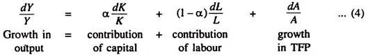
Thus, according to the GA method, there are three sources of growth as are captured by the key equation (4), viz., (i) changes in the amount of capital, (ii) changes in the amount of labour and (iii) changes in TFP. Since data on TFP are not readily available, we compute the growth in TFP by subtracting the first two terms on the r.h.s. of equation (4) from the 1.h.s.:

In this context dA/A is called the residual factor of growth in the sense that it cannot be explained by systematic changes in inputs. But it may be attributed to random variables such as a favourable technological change. Thus if 65% of a country’s growth rate is accounted for by the growth of labour force and capital stock, then it follows, by deduction, that the remaining 35% of its economic growth is due to increase in TFP. E.

Denison called it a measure of our ignorance. Modern economists call it the Solow residual because it was R.M. Solow (1924 -) who first showed how to compute it. In fact, in terms of the Solow model (to be discussed in this chapter) we find a close relation between growth in labour efficiency (E) to growth in TFP.

In Solow’s model

where (1- α) is labours share in total output. Thus technological change, as measured by the growth in the efficiency of labour, is proportional to technological change as measured by the Solow residual i.e., dA/A. Here α is the proportionality factor.

Since increased knowledge about production method (due to more investment in worker education and training) often raises TFP, the Solow residual is often used as a measure of technological progress. Anything which alters the relation between measured inputs and measured output will have an effect on TFP.

For example, if firms are forced to install new pollution, control equipment, MPK will fall and TFP will fall, too. Table 4.1 shows the steps involved in growth accounting approach.

Theory and Evidence:

Sources of productivity growth and reasons for its change have not yet been successfully isolated quantitatively. However, economic research has pointed out that business expendi­tures for research and development were consistently found to be positively associated with increases in output per unit of input in a large number of cases.

Periods of severe recession or of large variation in prices coincided with periods of slower growth in productivity.

We should not get the impression, however, that economists can calculate or measure the coefficient on capital growth in the growth accounting formula with much precision.

There is uncertainty about its size. It could be 1/4 or even 5/12. In any case, the growth accounting formula is a helpful rule-of-thumb to assist policy-makers in deciding what emphasis to place on capital versus technology when developing programmes to stimulate economic growth.

Prediction:

Unless productivity growth accelerates it is apprehended that prolonged periods of slow growth in real earnings and in per capita income will result. This will lead to deterioration in living standards even in advanced countries, not to speak of developing countries.

Policy Prescription:

The main policy approaches for raising productivity growth concern stimulation of investment in modern fixed capital, training and education, social infrastructure and development of new technologies as well as maintenance of economic stability. This has been demonstrated clearly by the newly industrialised countries of East Asia.

Case Example: A Tale of Two Countries:

The Growth Accounting (GA) formula can also be used to examine the very high-growth economies of East Asia. Consider Hong Kong and Singapore, for example. Both had approximately the same high rate of 5% per year productivity growth over the 1970s and 1980s.

But, by applying the GA formula some economists find that there is an enormous difference in how important technological change was compared to the growth of capital per worker in the two countries.

On the one hand, Hong Kong had a growth rate of technology that contributed almost 35% of the growth rate of output. Capital per worker contributed about 65% of growth. On the other hand, the growth accounting formula shows that Singapore had virtually no technological change during this period. It was generating the high growth rate solely through a very high growth rate of capital per worker.

Why the large difference in the role of technological change? The Singapore government encouraged firms to produce the very latest products. Perhaps this policy caused firms to switch too rapidly from one leading product to another and prevented them from learning to be more efficient in producing any given product.

Hong Kong did not follow such a policy. However, Hong Kong had a better-educated labour force, and this may have improved technology.

Examples:

1. Suppose capital’s share of output is 0.25 and labour’s share of output is 0.75

(a) Find the rate of growth of output dY/Y when the labour supply increases at a 1% rate, capital increases at a 4% rate, and total factor productivity increases at a 2% rate ? (b) What is the rate of growth of output (dY/Y) if the labour supply increases at a 4% rate, capital increases at a 1% rate, and factor productivity increases at a 2% rate ? (c) Explain the difference in the rate of growth in both the cases (a) and (b).

Solution:

(a) dY/Y equals dA/A + a = 0.75 (labour’s share of output). Thus, dY/Y =2% + 0.25(4%) + 0.75(1%) = 3,75%; output is increasing at a 3.75% rate.

(b) dY/Y = 2% + 0.25 (1%) + 0.75(4%) = 5.25%; output is increasing at a 5.25% rate.

(c) The impact of the growth of capital and labour upon the growth of output depends upon their relative importance in producing output as measured by their weighted share of income. Since labour’s share is three times that of capital, a 4% growth rate for labour contributes 3% to output growth, whereas a 4% growth rate for capital contributes 1% to output growth.

2. Suppose capital’s share of output is 0.25 and labour’s share of output is 0.75.

(a) Find the growth of total factor productivity dA/A when the labour supply increases 1%, capital increases 4% and output growth is 4%. (b) Find the growth of factor productivity dA/A when the labour supply increases 3%, capital increases 3%, and output growth is 4%. (c) Why is the TFP a residual?

Solution:

(a) dA/A equals dY/Y – a dK/K – (1 – a )dUL, where a = 0.25 and 1 – a = 0.75. Thus, dA/A = 4% – 0.25(4%) – 0.75(1%) = 2.25%.

(b) dA/A = 4% – 0.25(3%) – 0.75(3%) = 1.00%; productivity growth is 1.00%.

(c) Capital, labour and output are directly measured; TFP is not. It is residual since its contribution to output is inferred from the output change that cannot be explained by changes in labour and capital.

2. Suppose capital’s share of output is 0.25 and labour’s share of output is 0.75.

(a) Find the growth of total factor productivity dA/A when the labour supply increases

1%, capital increases 4% and output growth is 4%. (b) Find the growth of factor productivity dA/A when the labour supply increases 3%, capital increases 3%, and output growth is 4%. (c) Why is the TFP a residual?

Solution:

(a) dA/A equals dY/Y – α dK/K – (1 – α )dL/L, where α = 0.25 and 1 – α = 0.75. Thus, dA/A = 4% – 0.25(4%) – 0.75(1%) = 2.25%.

(b) dA/A = 4% – 0.25(3%) – 0.75(3%) = 1.00%; productivity growth is 1.00%.

(c) Capital, labour and output are directly measured; TFT is not. It is residual since its contribution to output is inferred from the output change that cannot be explained by changes in labour and capital.

Theories of Economic Growth:

The subject called ‘growth theory’ became popular in the post Second World War period (1939-45). Growth theories seek to explain the income differences among nations over time. Three main sources of growth are: (1) growth of the labour force, (2) capital accumulation and (3) technological progress.

The first two are sources of external growth and the third one which raises the productivity of existing resources — is the source of internal growth. In each Case the production possibilities curve (PPC) of society shifts to the right.

The most celebrated model of growth is no doubt the Harrod-Domar model. Harrod and Domar made the pioneering efforts to extend the basic Keynesian model of income and employment to study the dynamic problems of growth and development.

The Keynesian analysis was static. Growth theory explains why the national income of a country grows and why some economies grow faster than others. So Harrod and Domar broadened Keynesian analysis to describe changes in the economy over time. By developing such a model, Harrod and Domar made the Keynesian analysis dynamic.

Growth theorists use a long-run growth model to study the general upward path of the economy over time. The growth models focus on the amount of labour and capital that go into the production of goods and services. Labour and capital conjointly produce the economy’s output. Most of the output is consumed by households, the rest by businesses.

The analysis of long-run growth with the emphasis on flexible prices comes from classical macroeconomics. Classical macroeconomics is basically an application of supply-and-demand model of traditional microeconomics to the whole economy. The growth model builds on this analysis showing how the growth of capital and labour determines the growth of potential GDP.

Theories of economic growth are concerned with the rate of long-run equilibrium growth, that is, with the rate of growth of output that yields full employment of labour and capital. Rising unemployment would be accompanied by deficient demand and falling prices. On the other hand, underutilisation of the capital stock would drive profits and investment incentives down, reducing investments and the demand for output.

The principal theory of equilibrium economic growth is the neo-classical theory, presented in the form of a model by R. M. Solow, popularly known as the Solow model of economic growth. This model has been developed in the context of a closed economy (in which there is no foreign trade) without government. The model has fascinated economists since the second half of the 1950s.