The Marshallian Welfare Economics (With Diagram)

The Marshallian theory of economic welfare is based on his tool of consumer s surplus. Marshall begins with the individual consumer’s surplus or welfare and then makes the transition to the aggregate consumer’s surplus. To explain the aggregate welfare of the community, he uses his tax-bounty analysis. First, we explain the individual consumer’s surplus or welfare and then the aggregate economic welfare.

Marshall’s Individual Consumer’s Welfare:

Marshall explains the individual consumer’s welfare with his tool of consumer’s surplus. Marshall defines consumer’s surplus as “the excess of the price which he would be willing to pay rather than go without the thing, over that which he actually does pay, is the economic measure of this surplus satisfaction.”

The price which a consumer pays for a commodity like salt, match box, postcard, etc. is always less than what he is willing to pay for it so that the satisfaction which he gets from its purchase is more than the price paid for it and thus he derives a surplus satisfaction which increases his welfare. He explains the consumer’s surplus from a given change in price as the area between the demand curve and the price axis within a range of the price variation.

Explanation:

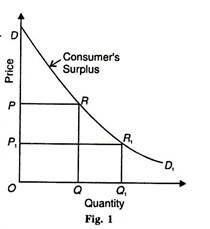
Consumer’s surplus is represented diagrammatically in Fig. 1 where DD₁ is the demand curve for the commodity. If OP is the price, OQ units of the commodity are purchased and the price paid is OP × OQ = area OQRP.

But the total amount of money, he is prepared to pay for OQ units is OQRD. 8 Therefore, consumer’s surplus =OQRD-OQRP = DRP. If the price of the commodity falls to OP₁, the consumer’s surplus increases to DR₁P₁ and conversely a rise in price would diminish it.

According to Prof. Hicks, this “Marshall’s measure” of the consumer’s surplus “involves nothing more introspective or subjective than the demand curve itself.” The area under the demand curve after deducting consumer’s expenditure on the commodity represents consumer’s surplus. This is based on the assumption of constant marginal utility of money for the consumer.

It is thus free from interpersonal comparisons of utility. So far we have studied the individual consumer’s surplus which is the sum total of the surplus from a number of commodities he buys, with a given money income.

By adding up consumer’s surplus from anyone commodity enjoyed by a number of individuals, the market consumers’ surplus for that commodity can be known. The demand schedule so formed will be the market demand curve. But it presupposes the nonexistence of interpersonal differences in customs, habits and incomes of the consumers.

Marshall’s Tax-Bounty Analysis of Aggregate Welfare:

The above analysis relates to the individual consumer’s surplus (welfare). In order to arrive at the aggregate consumers’ surplus, Marshall adds the individual consumer’s surpluses in a market. This he does by assuming that most markets are homogeneous with respect to the income class of the buyers and regards the individual buyer as a model representative of the group.

To get rid of the problem of interpersonal utility comparisons and value judgements, Marshall says that for practical purposes the area between the demand curve and the price is taken to be a good approximation of the sum of the individual consumers’ surpluses.

Marshall uses his tax-boundary analysis to explain the aggregate economic welfare. According to Marshall, aggregate economic welfare g D. can be increased by taxing diminishing returns industries and using the tax receipts to subsidies increasing returns industries. To arrive at this conclusion, he explains the following three possible cases.

Constant Returns:

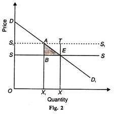
Marshall shows that a tax imposed on a commodity obeying the law of constant costs or constant returns results in a loss of consumer’s surplus greater than the amount of tax receipts, and conversely, a subsidy in this case exceeds the gain in consumers’ surplus. This is illustrated in Fig. 2, where SS is the supply curve of the commodity before the tax.

Since constant cost conditions prevail, the supply price is the same for all units of the commodity. Thus, the supply curve is perfectly elastic. DD₁ is the demand curve for the commodity. E is the initial equilibrium point where the consumers’ surplus is SDE.

Suppose, a uniform tax ТЕ per unit of the commodity bought is levied. The supply curve shifts up by the amount of the tax to S₁-S₁, parallel to the old supply curve SS. As a result, the loss of consumers’ surplus is the area SS₁AE (= SDE – S₁DA). The tax receipts to the government are equal to the area SS₁AB. Thus the loss of consumer’s surplus is greater than the gain to the government because SS₁AE > SS’AB.

The net loss of consumers’ surplus is the shaded area ABE. In the same way, if a subsidy shifts the long-run supply curve down from S₁S₁ to SS (whereby supply increases) the triangle ATE above the demand curve means the excess of subsidies paid out over consumers’ surplus gained.

Diminishing Returns:

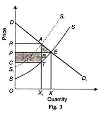
When the industry is operating under diminishing returns to scale or (increasing costs), the effects of a tax is not so certain. Whether the tax receipts will exceed the loss in consumers’ surplus will depend upon the steepness of the long-run supply curve.

This case is illustrated in Fig. 3 where the initial supply curve is SS. After the imposition of tax, it shifts to S₁S₁. The demand curve DD₁ intersects the supply curve SS at point E and the new supply curve at point .4. ТА per unit of tax is levied on OX₁ quantity of the product purchased and the total tax receipts are equal to the area С RAT and the loss in consumers’ surplus is RAEP. The receipts from tax shown as the shaded rectangle CPBT are greater than the net loss in consumers’ surplus, shown as the shaded triangle AEB.

Increasing Returns:

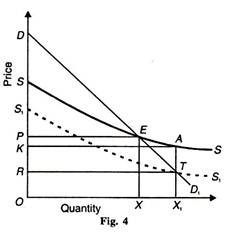
When the industry is operating under increasing returns to scale or diminishing costs, the long-run supply curve slopes downward as SS in Fig. 4. With the DD₁ demand curve, OX commodity is produced at the equilibrium point E. If a tax is levied, the cost of production will increase, the price of the commodity will rise and there will be loss in consumers’ surplus. (Not shown in the figure). However, the effect of a subsidy on a decreasing cost industry depends on the slope of the supply curve.

If the supply curve is less elastic, as shown in Fig. 4 the grant of AT amount of subsidy per unit of output to this industry will increase its output to OX₁ .The total amount of subsidy is RTAK and the gain in consumer’s surplus is RPET. As the area RPET > RTAK the gain in consumers’ surplus is greater than the amount of subsidy payment by the government. If the long-run supply curve is more elastic, as in the case of constant cost industry, subsidy payment will exceed consumers’ surplus even in diminishing cost industry.

Conclusion:

Marshall concludes that aggregate welfare can be increased if the government imposes a tax on diminishing returns or increasing cost industries (where tax receipts are greater than the loss in consumers’ surplus) and spends the proceeds to subsidies increasing returns or diminishing cost industries where the gain in consumers’ surplus is more than subsidy payments.