
In this article we will discuss about Maximisation of Social Welfare. After reading this article you will learn about: 1. Introduction to Maximisation of Social Welfare 2. Assumptions of Maximisation of Social Welfare 3. Explanation.
Introduction to Maximisation of Social Welfare:
Professor Bator in his paper “The Simple Analystics of Welfare Maximisation” has presented a more thorough and systematic analysis of the problem of social welfare maximisation. It is a summary of the static long-run general equilibrium conditions of a perfectly competitive economy.
It combines the Pareto optimality conditions with the social welfare function and provides a determinate and unique solution to the problem of maximisation of social welfare.
Assumptions of Maximisation of Social Welfare:
The analysis of maximisation of social welfare is based on the following assumptions:
ADVERTISEMENTS:
1. There are two homogeneous and perfectly divisible inputs, labour (L) and capital (K). The two are supplied in fixed quantities.
2. Only two homogeneous goods, X and Y are produced in the economy. The production function for each good is given and does not change. Each production function is smooth, shows constant returns to scale and diminishing marginal rate of technical substitution along any isoquant which means that the isoquants are convex to the origin.
3. There are two individuals, A and B, in the economy. Each has a set of smooth indifference curves convex to the origin which reflect consistent ordinal preference functions.
4. There is a social welfare function that is based on the positions of A and B in their own preference scale, i.e. W = W (WA, WB). It presents a unique preference ordering of all possible situations,
Explanation to Maximisation of Social Welfare:
ADVERTISEMENTS:
Given these assumptions, the problem is to determine the welfare maximising values of:
(i) The input of labour into the production of X and Y,
(ii) The input of capital into the production of X and Y;
(iii) The total amount of X and Y produced; and
ADVERTISEMENTS:
(iv) The distribution of X and Y between the two individuals A and B.
These steps are analysed as under:
From the Production Function to the Production Possibility Curve:
The box diagram Figure 1 explains the general equilibrium of production. There are fixed amounts of two inputs, labour (L) and capital (K), available to the economy for the production of two goods X and Y. Ox is the origin of input labour which is measured along the horizontal axis, and Oy of input capital which is measured along the vertical axis. The horizontal sides of the two axes, Ox and O represent good X and the vertical sides good Y.
The production function for each good is given by smooth isoquants which are characterised by constant returns to scale and diminishing marginal rates of technical substitution (MRTS). These isoquants are X1 ,X2 and X3 for good X for which Ox is the origin, and Y1, Y2 and Y3 for good for which Ox is the origin.
At points P1 Q 1 and R1 an isoquant of good X is tangent to an isoquant of good Y, and so satisfies the condition MRTSLK – yMRTSLK. By joining these tangency points leads to the production contract curve Ox P1 Q1 R1 Oy in input space. The various points on this contract curve are of efficiency locus where an increase in the production of X implies a necessary reduction in the output of Y.
From this production contract curve, we can trace the production possibility curve or transformation curve in the output space from the input space. The production possibility curve associated with the contract curve Ox P1 Q1 R1 Ox of Figure 2 is plotted as TC in Figure 2 This curve shows the various combinations of X and Y can be produced with fixed amounts of labour and capital. Consider point P1 on the contract curve and input space of Figure 60.1.
If the isoquant Y3 represents 600 units of input Y, and X1. 100 units of X they are mapped in the output space as point P in Figure 2. Similarly points Q1 and R1, of Figure 1 are traced in the output space as points Q and R respectively in Figure 60.2.
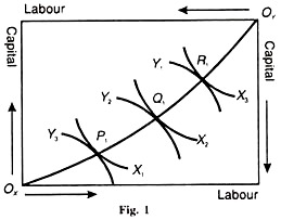
By joining points P, Q and R, we derive the production possibility curve TC for good X and Y. With given amounts of labour and capital and fixed technology the economy cannot attain any point above the TC curve. Nor can it have a point inside the TC curve for that will mean underutilization of the two factor endowments.
ADVERTISEMENTS:
The economy must, therefore, be on the TC curve to maximise the community welfare. Further, the slope of any point on the production possibility curve of Figure 60 2 reflects the marginal rate of transformation (MRT) of X into Y. In other words, it indicates by how much the output of Y must be reduced by transferring enough capital and labour to produce one more unit of X.
From the Production Possibility Curve to the Grand Utility Possibility Curve:
The next step is to specify general equilibrium of exchange in the economy consisting of two individuals A and В and two goods X and Y. For this purpose, we derive the grand utility possibility curve from the production possibility curve. This is done by mapping the consumption contract curve from the output space of the production possibility curve TC of Figure 2. in to a utility space.
ADVERTISEMENTS:

Select any point Q on the transformation curve TC in Figure 2 so that the total outputs of X and У are OX and OY respectively. These outputs of X and Y determine the volume of the two goods available to A and B. These outputs, in turn, determine the dimensions of an Edge worth box diagram for exchange.
Drop perpendiculars X and Y from Q on the two axis. Now О becomes the origin of consumer A. Let it be OA. Similarly, point Q becomes the origin of consumer B. Let it be OB. Since each individual has a well-defined preference function, indifference curves of A and В are drawn in the exchange box. Curves A1, A2 and A3 represent A’s preference field, and В1 В2 and B3 are В’s. The locus of tangencies of the indifference curves of A and В are E, F and G By joining these points, we get a consumption contract curve ОAEFGОB.
This curve is the locus of the various points of tangencies which shows the various positions of exchange that equalize the marginal rates of substitution of point of the consumption contract curve satisfies the optimum conditions of exchange. But a movement along the contract curve makes one individual better off than the other. Thus each point on the contract curve is a Pareto optimality point.
ADVERTISEMENTS:
By observing the utility levels for A and В at each point on the contract curve Figure 2 we can derive the utility possibility curve or frontier relative to the output point Q on the transformation curve TC. The utility curve relative to Q is plotted as U1U2 in Figure 3.

Point E on this curve corresponds to point E on A1 B3 curves in Figure 2. Point E can be arrived at in this way. If the utility of curve A1 is 100 units and of В curve 450 units with the horizontal axis referring to A’s utility and the vertical axis B’s utility, we get point E1 .Point F1 corresponds to point F on A2, В2 curves, and G1, corresponds to point G on A3 B1, curves. By joining these points, we get the utility possibility curve U1U2 as shown in Figure 3. This curve is the locus of points of maximum utility for A for any other level of utility for B.
The condition for welfare maximisation also requires the general Utility equilibrium of exchange and production simultaneously. This condition implies that the marginal rate of substitution of X and Y must equal the marginal rate of transformation between the two. There is, however, one point out of the many points on the utility possibility curve that satisfies this condition. It is point F, on the U1, U2 curve in Figure 3 which corresponds to point F on the contract curve in Figure 2. It is found out by drawing a tangent aa at Q on the TC curve in Figure 2.
The slope of this tangent at Q represents the marginal rate of transformation between X and Y. The slope of the tangent bb at F in the box diagram represents the marginal rate of substitution for X and у by individuals A and B. Since the two tangents aa and bb are parallel to each other, point F in Figure 2 and point F1 in Figure 60.3 satisfy the condition of simultaneous general equilibrium of exchange and production, i.e. AMRSxy = BMRSxy= MRTxy.
By taking any other point P or R on the production possibility curve TC of Figure 2, we can construct another Edge worth box diagram and consumption contract curve. From this another utility possibility curve can be drawn and another point of Pareto optimum in exchange and production can be found. Let such a utility possibility curve be USU4 with the corresponding point A, as shown in Figure 4.
ADVERTISEMENTS:
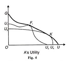
The utility possibility curve U.U, of figure 60.3 with the Pareto optimum point F, is also drawn in this figure. By joining these points F, and K, we derive GU as the grand utility possibility curve. The grand utility possibility curve is the locus of Pareto optimum points of exchange and production.
From the Grand Utility Possibility Curve to the Point of Constrained Bliss:
In order to find out which of the Paretian optimum points on the grand utility possibility curve represents the maximum social welfare, we have to draw a social welfare function. Figure 5 shows W W1 and W as three social welfare functions or social-indifference curves of the society. Each social welfare function shows the various combinations of A’s utility and B’s utility which give the same level of satisfaction.
But a movement along a social welfare function makes one individual better off and the other worse off. Thus a social welfare function involves interpersonal comparisons of utility.
Assuming that W, W, and W2 are the social welfare curves which exist for the society, social welfare will be maximised where the grand utility possibility curve is tangent to a social welfare curve, In Figure 5, F is the point of maximum social welfare as determined by that tangency of W, curve and GU curve. This is known as the point of “constrained bliss” because a movement away from point F along the GU curve will reduce total social welfare.

Take point P or R on the grand possibility curve GU. They represent a lower level of welfare because they are on the lower social welfare curve W. All points which are below the point of constrained bliss F are of non-Pareto optimality. And all points above this point such as С on the W curve are beyond the reach of the society because of given factor endowment and technology.
Thus point F is of maximum social welfare where the general equilibrium conditions of production, exchange, and production and exchange are simultaneously satisfied.