Economic Theory of Index Numbers: Assessing Changes in Standards of Living

A significant use of indifference curve analysis is made in the economic theory of index numbers.

First, let us make it clear what is the index number problem in economic theory.

To make the analysis simple let us assume an individual consumer purchases two commodities, X and Y, in two different time periods, zero and one.

In period zero, the consumer purchases 25 units of good X at price Rs. 10 per unit and 15 units of good Y at price Rs. 12 per unit. Suppose the prices of goods X and Y change in period one and at price of X equal to Rs. 15 the consumer purchases 20 units of good X, and at price of Y equal to Rs. 9 he purchases 22 units of good Y.

Thus in period one the quantity purchased of good X has fallen while the quantity purchased of good Y has increased. Now, the problem of index number is whether the economic welfare or standard of living of the individuals has increased or decreased in period one as compared with period zero. If indifference map of individual is known, then with its aid we can know whether welfare of the individual has increased or decreased.

Let us restate the index number problem in notational form. Suppose in period zero individual buys x° quantity of commodity X at price p⁰_x and y⁰ quantity of commodity Y at price P°_y. Similarly, in period one, individual purchases X₁ quantity of commodity X at price P¹_x and Y¹ quantity of commodity Y at price p¹_y.

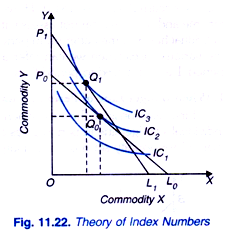
We have to assess whether the standard of living or welfare of the individual has increased or decreased during the period one as compared with period zero with the change in relative prices and income of the individual. To make this assessment we assume that individual’s tastes and preferences, that is, his indifference map remains constant and unchanged over the time period under consideration. Indifference curves IC₁, IC₂ and IC₃ depict the indifference map of the individual between commodity X and Y.

In the period zero (called the base period), individual’s given money income and the Prices P⁰_x and P⁰_y give rise to the budget line P₀L₀. It will be seen from Figure 11.22 that with budget line P₀L₀ individual is in equilibrium at point Q₀ on indifference curve IC₂. As a result of the changes in income and prices of goods in period one, the budget line changes to P₁L₁ (the relative price of X has risen).

The new budget line P₁L₁ is tangent to indifference curves IC₃ at point Q₁ where the individual is now in equilibrium. It will be seen from the figure that in this new equilibrium position reached after the change in income and prices of goods and the consequent changes in the bundle of goods X and Y from Q₀ to Q₁, the individual becomes better off (that is, his standard of living in terms of utility or satisfaction has increased), since he has shifted to a higher indifference curve IC₃ from IC₂. In other words, he has enjoyed a gain in real income by the above changes in prices and quantities, for they have pushed him to a higher indifference curve. But it should be noted that we are able to judge the increment in real income or economic welfare only when the indifference-curves map of the individual is actually known. However, if the indifference curves are not known, as is usually the case, and we know only the budget lines and the consumption points Q₀ and Q₁, we cannot assess with the aid of indifference curve analysis whether the real income, or standard of living or welfare of the individual has increased or decreased by the above stated changes in prices and quantities purchased of .the commodities, for in the absence of indifference curves depending upon his subjective preferences we cannot know whether or not individual has shifted to a higher indifference curve.

Fortunately, in several cases even in the absence of knowledge about individual’s indifference curves we can judge whether with the changes in income and relative prices, he has become better off in period 1 as compared to the base period by simply observing the behaviour of the individual regarding his choice of bundle of goods in different periods.

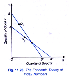
In this analysis only assumption which we make is that the individual makes rational choice. Consider the situation depicted in Figure 11.22 now reproduced in Figure 11.23 without the indifference curves. With the given income and prices of goods in period 0 (i.e. the base period) the budget line is A A’. Suppose with a certain change in income and price of goods, the individual’s budget line becomes BB’ in period 1.

It is observed that the consumer chooses bundle of goods Q₀ in period 0 on the budget line AA’ and the bundle Q₁ in period 1 on budget line BB’. Now, we have to assess whether the consumer has become better off in period 1 as compared to period 0. It will be seen that in period 1 the bundle Q₀ is available (that is, Q₀ lies within market opportunity set or budget space of the budget line BB’ of period 1 but the consumer actually chooses the bundle Q₁ implying that he prefers bundle Q₁.

In other words, he has become better off (that is, his real income has increased) in period 1 as a result of changes in prices and income occurred since period 0. We cannot assess without the knowledge of indifference curves whether the individual has become better off in period 1 as compared to the base period.We explain below the various cases when we can infer about whether the consumer has become better off in period 1 as compared to period 0 as a result of changes in income and prices.

1. When Budget Line of Period 1 Lies Entirely Outward to the Base Period’s Budget Line:

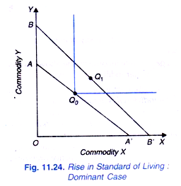
First, we consider the case when prices and money income have so changed that the individual’s budget line in period 1 lies outward to the budget line in period 0 implying that his market opportunity set has been enlarged. For instance, consider Figure 11.24 where AA’ is the budget line in the base period and with the change in income and relative prices of goods, the budget line in period 1 shifts entirely outward to the position BE’ with greater intercepts on both the axes.

Note that we are assuming that both the commodities are ‘goods’ and further that the consumer behaves rationally, that is, he prefers more to less of a good. Suppose the consumer chooses bundle Q₀ on budget line AA’ in period 0 and bundle Q₁ on budget line BB in period 1. Since bundle Q₁ in period 1 is lying in the north east of Q₀ contains more of both the goods. We can unambiguously say that he has become better off or his standard of living has risen in period 1 as compared to the period 0.

2. Budget Line of period 1 intersects the Budget line of period:

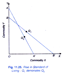
When income and relative prices change in such a way that budget line of period 1 intersects the budget line of period 0, it is somewhat difficult to assess whether the consumer has become better off in period 1. However, in some cases we can say unambiguously whether or not there is improvement in standard of living of consumer in period 1.

For instance, consider Figure 11.25 where AA’ is the budget line in the base period and with changes in income and relative prices, budget line in period 1 becomes BB’ which intersects the base- period budget line AA’. In the base period the consumer chooses bundle Q₀ on the budget line AA’ and in period 1 his choice is the bundle Q₁ lying north east of the bundle Q₀. It will be noticed that the bundle Q₁ contains more of both goods X and Y as compared to Q₀ in the base period. We can therefore say unambiguously that his standard of living has improved in period 1.

3. Budget Lines of the Two Periods Intersect: The Ambiguous Cases:

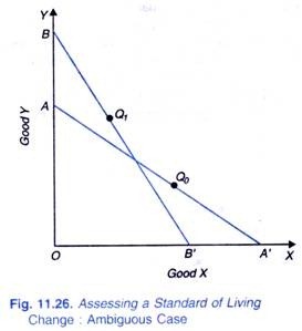
The situation depicted in Figure 11.26 poses a difficult problem for assessing whether or not there is improvement in the standard of living in period 1. In this case, as will be seen from Figure 11.26, the budget lines intersect and the consumer chooses the bundle Q₀ in period 0 and the bundle Q₁ in period 1 which lies to the north-west of Q₀.

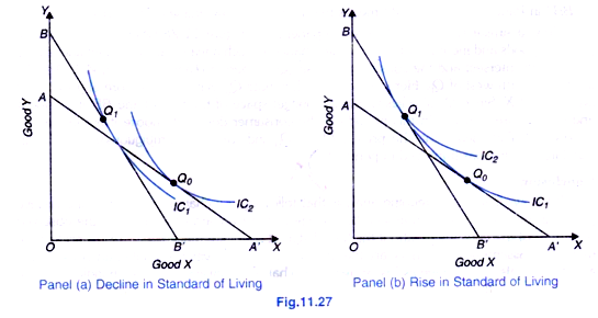
This is an ambiguous case because without the knowledge of consumer’s indifference curves we cannot infer form his observed behaviour whether or not he has become better off. This is because both situations are possible depending on the shapes and location of his indifference curves.

As will be seen from Figure 11.27 (panels a and b) with Q₁ living northwest of Q₀, it would be possible to construct indifference curves so that Q₀ lies on a higher indifference curve than Q₁ as in (panel a) but is equally possible to construct indifference curves so that Q₁ of period 1 lies on a higher indifference curve than Q₀ (as in panel b). If the indifference curves of our consumer are those that are depicted in panel (a), then change in situation from AA’ to BB’ will make him worse off and if his indifference curves are such that are shown in panel b, then he would become better off in period 1.

4. Budget Lines of the Two Periods Intersect: Non-Dominant Cases:

There are certain situations when we cannot at first glance conclude unambiguously whether or not individual has become better off in period 1. For example, consider the situation depicted in Figure 11.28. To start with, consumer chooses Q₀ on AA’ in period 0 and with changes in income and relative prices he chooses Q₁ on BB in period 1. The dominance criteria to assess improvement in standard of living cannot be applied.

Here bundle Q₁ of period 1 contains more of X but less of Y as compared to the bundle Q₀ in the base period (Note that neither Q₁ dominates Q₀ nor Q₀ dominates Q₁), Nevertheless, we can infer about the change in standard of living in period 1 from his observed behaviour and attainable bundles in each period.

In period 0, the budget line is AA’ and the consumer chooses Q₀ when Q₁ is attainable, that is, Q₁ lies within the budget space or market opportunity set of the budget line AA’, thus the consumer could have chosen Q₁ but, instead he chose Q₀ implying thereby that he prefers bundle Q₀ to Q₁. Thus the change in situation from Q₀ on AA’ to Q₁ on BB’ in Panel (a) of Fig. 11.28 means that he has become worse off in period 1.

Now, a similar situation is depicted in panel (b) of Figure 11.28 were also the relative prices of goods and income of the consumer change in such a way that the budget lines of the two periods intersect and the consumer chooses Q₀ in period 0 and Q₁ in period 1. And lies to the north-west of Q₀.

Here Q₁ does not dominate Q₀ as it contains more of good Y but less of good X. Since Q₀ also lies within the budget space of the budget line BB in period 1 and is therefore available in this period but the consumer does not choose it but instead he chooses Q₁. This means that he prefers Q₁ to Q₀ and we can unambiguously say that his standard of living has improved in period 1.