Algebraic Solution to the Simple Keynesian Model

Algebraic Solution to the Simple Keynesian Model | Keynes’s General Theory

Article shared by:

Let us make an in-depth study of the algebraic solution to the simple Keynesian Model.

The issue Keynes was addressing is what happens if planned aggregate production and planned aggregate expenditures are not equal—how both of them will adjust until they are equal. When they are equal we have:

C + S = C + I

or, subtracting C from both sides,

ADVERTISEMENTS:

S = I

The equations (1) and (2) represent the equilibrium condition. It tells us that as long as planned savings are greater than planned investment, inventories will be building up and firms will be reducing production so that their inventories are at the desired level.

Similarly as long as planned savings are less than planned investment, inventories will be lower than desired and firms will be increasing production so that their output plans are satisfied. It is only when planned saving equals planned investment will there be no motivation to change the output. We define this as the equilibrium state.

The four equations spelling out the simple Keynesian model are the following:

ADVERTISEMENTS:

C = a + b Y (Consumption expenditures)

I = I₀ (Investment expenditures)

Y = C + S (a 45° line representing aggregate production)

C + S = C + I (the equilibrium condition)

ADVERTISEMENTS:

or S = I

We can solve this system of equations to obtain an expression for the value of Y as under:

The equilibrium condition is expressed as

S = I₀

We can add the relation about consumption expenditures into equation (3) on both sides and we get

a + bY + I₀ = C + I = Y

Subtracting b Y from both sides of equation (4), we have

a + I₀ = Y-bY

Factoring Y on the right-hand side yields

ADVERTISEMENTS:

a + I₀=Y(I-b)

Dividing both sides by (1 – b) we have

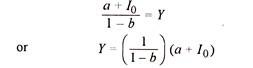
The last equation is called a reduced form equation because it embodies all the information in the four equations of the Keynesian model in one equation. It shows us at one glance all the variables on which income depends. The second term on the right, (a + I₀), contains all autonomous variables and is called autonomous expenditure. The first term on the right, 1/ (1 – b) or 1 IMPS, is called the multiplier. It tells us by how much we must multiply autonomous expenditure to determine the level of income in the economy.