Stability of Equilibrium (With Diagram) | Simple Keynesian Model

Let us make an in-depth study of the Stability of Equilibrium.

The assumption that 0 < b < 1 is crucial for establishing stability in SKM.

Stability in this context refers to a stable equilibrium position in the commodity market.

The stability condition is that the slope of the C + I + G schedule has to be less than unity.

For the sake of simplicity we ignore government expenditure and taxes. So we are now examining the SKM without government.

In a two-sector economy the slope of C + I schedule has to be less than unity. Here the C + I schedule is parallel to C schedule since I is autonomous. Hence the slope of the C + I schedule is the same as the slope of the C schedule (since the slope of I schedule is zero). Thus for a given level of autonomous investment the equilibrium value of Y is determined by the consumption function.

If the slope of the consumption function is less than 1, the slope of the C + I schedule will also be less than 1. This will then be less than the slope of the income line Y = C + S (ignoring taxes). And equilibrium will be stable as shown in Fig. 8.6(a). Otherwise it will be unstable as shown in Fig. 816(b). This point may now be proved.

In SKM, AD is equal to C + I̅ and AS is equal to Y. Suppose excess demand (E) is equal to AD – AS, i.e., E = C + I̅ – Y. Here E is a function of Y. According to the Walrasian stability Condition the commodity market will be stable if

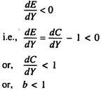
Here b is MPC.

If b > 1, the C + I schedule will intersect the income line from below and equilibrium will be unstable. Any deviation of Y_e in either direction will be cumulative in nature as shown in Fig. 8.6.

i. The Stability Condition:

The stability condition in the SKM is that the MPC(b) should lie in-between zero and one. It has to be greater than zero and less than one. We may now rigorously demonstrate the income path in SKM with a lagged consumption function.

We know that the Keynesian consumption function is linear. If we assume that there is one period lag in the consumption function then we can express the function as C_t = a + bY_t-1 where is the last period’s income, a is the intercept of the function (showing autonomous or income-independent consumption) and b is the MPC (0 < b < 1). Since in SKM all investment is autonomous and thus remains constant at all levels of income we write I_t, = I̅. Now equilibrium in the goods (commodity) market requires that Y_t = C_t + I_t, or, Y_t, = a + bY_t-1 + I̅. or, Y_t = bY_t-1 + (a + I̅).

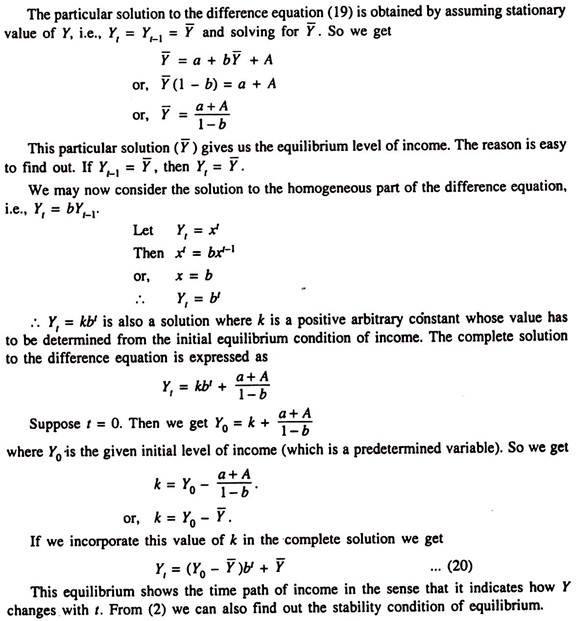
From the particular solution to this first order linear homogeneous difference equation, we arrive at the equilibrium value of national income (Y_e) in SKM. Assuming income to remain constant overtime we put Y_t = Y_t-1 = Y_e. Therefore we get Y_e = bY_e + a + I̅.

Here Y_e is the equilibrium value of income. Since Y_e is assumed to remain unchanged period after period, if Y_t-1, = Y_e then Y_t will also be equal to Y_e. Thus if Y was in equilibrium last year (t – 1) then it will also be in equilibrium in the current year. Similarly, if Y is in equilibrium in the current year, it will also be in equilibrium next year.

ii. The Derivation of the Stability Condition in SKM:

The equilibrium level of income is said to be stable if any deviation from it tends to create forces that bring actual income back to the equilibrium level. Let us suppose, in the context of SKM, that in period (t – 1) actual income exceeds its equilibrium level. Suppose Y_t-1, = Y_e + k where k > 0. So we have

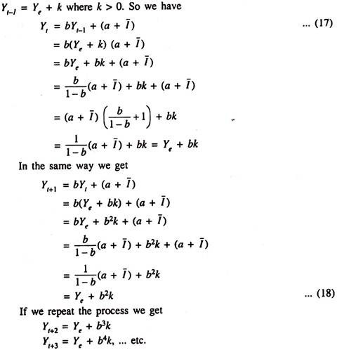
This means that the income rises in different time periods in this dynamic SKM (where time enters the analysis as an important variable) and will be (Y_e + k), (Y_e + bk), (Y_e + bk²), (Y_e + b²k),… etc. Now if the MPC(b) is greater than 1, then we have k < bk < b²k< b³k …

This simply implies that if in any period actual income goes above its equilibrium level then the gap between the two (i.e., the excess of actual income over the equilibrium income will continue to increase with the passage of time. But if MPC(b) is less than 1 we have

k > bk > b²k > b³k …

In this case the gap between the two (i.e., the excess of actual income over equilibrium income) becomes gradually smaller and smaller. Thus if b > 1 the equilibrium level of income in SKM is unstable, in the sense that any deviation of actual income (Y) from its equilibrium level (Y_e) does not bring Y back to Y_e. But if b is less than 1, Y_e is stable because in case of any deviation of Y from Y_e, Y moves toward Y_e in the next and subsequent periods. It is also quite obvious that if k < 0, i.e., < Y_t-1 Y_e, then the gap between the two (deficiency of Y from Y_e) will increase b < 1 and the gap will become smaller and smaller and ultimately disappear if b < 1.

If b = 1 we have Y_t – Y_t-1 + (a + I̅).

In this case if we assume that (a + I̅) = 0, i.e., there is no autonomous (income independent) expenditure, then Y_t = Y_t-1 [from equation (1)]. If such a restrictive assumption is made, the level of income (Y) remains constant in all time periods. This means that the economy, does not grow. It is in a stationary state where national income remains constant. Some economists even call this type of equilibrium behaviour by the name ‘neutral equilibrium’.

However, if (a + I̅) is positive or negative, equilibrium will not even exist. If (a + I̅) > 0, then income in period T will be greater than Y_t-1 by (a + I̅), in which case Y will continue to grow without limit. It will explode. In contrast if (a + I̅) < 0, Y will fall without limit. It will fall toward zero.

So the basic point to note is that if and only if b < 1 the income path in SKM will be stable.

iii. Dynamic Analysis:

A. Consumption Lag of One Period:

Although the SKM is static in nature, we can extend it to make a dynamic analysis of the income path by considering a lagged consumption function. This means that consumption in the current period (r) depends on the income of the last period (t – 1). So the Keynesian linear consumption function can be expressed as C_t = a + bY_t-1 where a is the intercept (a positive constant) and b is the slope (the MPC which is also a positive constant).

We continue to assume that all investment is autonomous and hence independent of income. So

I_t, = I̅_t. Thus the income equation in SKM is

Y_t, = a + bY_t-1 + I̅_t … (19)

The solution of this first order linear homogeneous difference equation gives the time path of income. This approach follows from the assumption that there is a one period consumption lag.

B. Production Lag of One Period:

Now we can adopt an alternative approach to Keynesian dynamics by assuming a production lag of one period. But there is no consumption lag. So we get

Y_t = C_t-1 + I_t-1 (where C_t-1 = a + bY_t-1 since there is no consumption lag now)

Y_t = a + bY_t-1 + I_t-1

= a + bY_t-1 + A where A = I_t-1 i.e., output in the current period is equal to aggregate demand of the last period.

iv. Two-part solution to the difference equation:

In this case also b has to be less than 1 in which case as t → ∝, b^t = 0 in the limit and Y_t → Y̅, even if Y₀ ≠ Y̅. This means that even if the initial level of income is different from the equilibrium level of income, then actual income will tend towards equilibrium value over time. If, however, b > 1, then as t ∝, b^t will also approach ∝, in which case the initial level of income will gradually diverge away and away from its equilibrium value. This means that the income path in SKM will be unstable.

Two possible income paths in Keynesian dynamic model are shown in Fig. 8.7. Now we show time on the horizontal axis and income on the vertical axis.

In Fig. 8.7(a) we assume that b < 1. Therefore if Y₀ > Y, then Y_t comes closer and closer to Y over time. Conversely, if Y₀ < Y then Y_t increases steadily and gradually moves toward Y with the passage of time. Thus the equilibrium income is stable.

In Fig. 8.7(b) we assume that b > 1. Therefore if Y₀ > Y, then income will continue to increase with the passage of time. This means that there will be no limit to the increase in income. Contrarily if Y₀ < Y actual income will continue to fall over time.

So there will be no limit to the fall in income. In this case actual income will move further and further away from its equilibrium value. In other words, the deviation from equilibrium becomes cumulative and equilibrium is unstable.

v. Induced Investment and Stability of Equilibrium:

We now relax the assumption that all investment is autonomous. We now assume that investment is partly autonomous and partly induced. Thus we can write

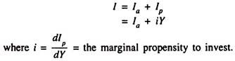
In this case the investment demand schedule, instead of being horizontal throughout will be upward sloping from left to right and its slope is the marginal propensity to invest (MPI) which is positive. The MPI is defined as the ratio of the change in investment to the change in national income which brings it about.

In this case, change in income leads to a change in investment while in the original SKM investment has no relation to income. Now that investment has an induced component also, we have to modify the stability condition of SKM.

In Fig. 8.8(a) we see that equilibrium income is stable. If there is any deviation of point E, Y will fall since MPI > MPS and Y will come back to the original level. In Fig 8.8(b) we see that equilibrium income is unstable. If there is any deviation of point E, Y will continue to move further and further away from Y_e.

Thus the condition of stability in this context is that MPI > MPS, i.e., the slope of the saving (S) schedule has to be less than that of the investment (I) schedule.

vi. Two Related Points:

1. Shift vs. Change in Slope:

If there is a change in any of the autonomous components of DE = C + I + G = a + bY- bT + I + G, the DE schedule will shift up or down. The autonomous components of E are a, -bT, I and G. There is a change in the slope of the DE schedule if Y changes. The slope of DE is b which is MPC (= ΔC/ΔY) which indicates how C and hence DE will change when income changes. If b increases (falls) the E schedule becomes steeper (flatter).

2. Two Components of Equilibrium Income:

The essence of the process of income determination in the context of SKM is captured by the following equation:

Y̅ = 1/1- b(a – bT + I + G) …(21)

So, equilibrium income = (autonomous expenditure multiplier) x (autonomous expen­ditures).

Here 1/(1 – b) is the autonomous expenditure multiplier. Here ‘b’ is the MPC and (1 – b) is the MPS. So the multiplier is the reciprocal of the MPS. Since MPC < 1, the multiplier is a number which is greater than 1. If b = 0.5, m = 2; if b = 0.8, m = 5. Thus if b increases m also increases.

The term ‘autonomous expenditure multiplier’ is derived from the fact that every rupee of autonomous expenditure is multiplied by this number to find out its contribution to equilibrium income.

The second component of equation (21) indicates the level of autonomous expenditures which is determined by factors other than current income. Here I and G are fully autonomous. But C is partly autonomous and partly induced. The terms related to C but unrelated to Y are a and – bT.

These two terms measure the autonomous component of consumption expenditures (a) and the autonomous effect of tax collections on aggregate demand (- bT), which also works through consumption. Since these two terms affect the amount of consumption for a given level of income (Y) and are not themselves determined by income, they are treated as autonomous component of C.