Simple Keynesian Model (SKM): Assumptions, Conditions and Defects

Let us make an in-depth study of the Simple Keynesian Model (SKM). After reading this article you will learn about: 1. Assumptions of the Simple Keynesian Model 2. Conditions for Equilibrium of SKM 3. Defects of SKM.

Assumptions of the Simple Keynesian Model:

The simple Keynesian model of income determination (henceforth the SKM) is based on the following assumptions:

1. Demand creates its own supply.

2. The aggregate price level remains fixed. This means that all variables are real variables and all changes are in real terms.

Therefore if aggregate demand increases, output will increase, prices remaining the same. And due to the existence of excess production capacity and unemployed resources (especially manpower) the economy will reach the point of full employment — if there is sufficient demand stimulation.

3. The economy has excess production capacity.

4. The economy is closed — there is no export and import.

5. There is no retained earnings. All profits are assumed to be distributed as dividends among the shareholders.

6. Firms are assumed to make no tax payments; all taxes are paid by households. The central proposition of the simple Keynesian model (the SKM) is that national output (income) reaches its equilibrium value when output is equal to aggregate demand.

In the SKM the condition for equilibrium can be expressed as:

Y = E – (1)

where Y is equal to total output (GDP) and E equals aggregate demand or desired expenditure on output. Aggregate demand or desired expenditure (E) has three components, viz., household consumption (Q, derived business investment demand (I) and government demand for (currently produced) goods and services. Thus the equilibrium condition of national income in a closed three-sector economy is

Y = E = C + I + G … (2)

This means that income received (K) is equal to desired expenditure (E). Here we do not distinguish between gross and net investment. So we ignore depreciation. Moreover we take GDP and national income as equivalent concepts. Thus, we ignore net indirect business, taxes — which cause discrepancy between the two totals.

Since national product (output) Y also measures national income, we can write

Y = C + S + T … (3)

This equation is basically an identity. It suggests that national income, all of which is assumed to be paid out to households in the form of factor incomes (such as rents, wages, interest and dividends) is partly consumed (C) partly saved (S) and partly paid in taxes (T).

Moreover, since Y is national product, we can write

Y = C + l_r+ G … (4)

This means that national product is equal to consumption plus realised investment (I_r) plus government spending.

From the definitions given in equation (3) and (4) we can rewrite the condition for equilibrium income given in equation (2) in two alternative ways.

From equation (2) we have Y = C + I + G in equilibrium, and from equation (3) we have Y = C + S + T, which is a definitional identity. In equilibrium, therefore, we have

C + S + T = Y = C + I + G … (5)

or, S + T = I + G,

In a like manner, from equations (2) and (4) we can express the equilibrium condition as

C + I_r + G = Y= C + I + G

or, by cancelling common terms, I_r = I … (6)

Conditions for Equilibrium of SKM:

Thus, there are three equivalent ways to state the condition for equilibrium in the SKM:

Y = C + I + G … (2)

S + T = I + G … (5)

I_r = I – (6)

These conditions are illustrated in Fig. 8.1. which is a circular flow diagram of income and output for a three-sector economy:

The revenue of the business sector is used for paying rent, wages, interest and dividends to the household sector. A portion of income received by the household sector (10 is used

by the households for consumption (C) which goes to the business sector as income. Another portion which is saved (S) goes to the business sector as investment (I) sector And the last portion goes to the government in the form of taxes (T) which finance government expenditure (G)which, in its turn, is spent on goods and services produced in the business sector.

Injections and Leakages:

In this context we draw a distinction between injections and leakages. Anything which exerts an expansionary pressure on national income is an injection and anything which exerts a contractionary pressure on national income is a leakage. Investment and government expenditure are injections into the circular flow of income, while savings (S) and taxes (T) are leakages from the circular flow of income.

Examination of the Three Equilibrium Conditions:

The three equilibrium conditions of national income given by equations (2), (5) and (6) may now be examined in detail. Production of a certain level of output, Y. generates he same amount of income to households. A portion of this income directly comes back to the firms as demand for consumption goods.

National output will reach its equilibrium level if this demand (C), when added to desired investment expenditure of firms (I) and government spending (G), produces a total demand equal to Y — that is, if

Y = C + I + G

The second equilibrium condition of income

S + T = I + G

suggests that a flow rate of output will be an equilibrium rate if the sum-total of leakages (S + T) is just balanced by the sum-total of injections (I + G).

This condition ensures that the amount of income households does not spend on output (S + T) and, therefore, the amount of output that is produced but not sold to households (Y – C = S + T)is exactly equal to the amount the other two sectors wish to buy (I + G). Thus total output equals aggregate demand.

Equation (6) states that in equilibrium desired (planned) investment must equal realised (actual) investment. What is the significance of the divergence of desired investment from realised investment? Total business investment has two broad components viz., fixed asset investment (or business spending on plant, equipment and machinery) and inventory investment (or increase or decrease in the stocks of finished goods and raw materials).

It is quite reasonable to assume that desired spending on plant and equipment equal actual spending. But desired inventory investment varies from realised inventory investment, n national income accounts, all goods that are produced by a firm and not sold are treated as inventory investment – whether such investment was intended or not.

In order to realise the difference between realised and intended investment totals, we have to see what happens when a level of output (Y = C + I_r + G) is produced that exceeds aggregate demand (Y = C + I + G).

In this case we have the following inequality:

Y > E

C + I_r + G > C + I + G > …(7)

I_r > I

where I_r – I is the undesired (unintended) accumulation of inventory. The excess of I_r over unintended inventory accumulation. It indicates the amount by which output exceeds aggregate demand, i.e., the output which will remain unsold over and above the amount of inventory investment the firms desired.

In the opposite situation, if aggregate demand exceeds output, we have

E > Y … (g)

C + I + G > C + I_r + G

I > I_r

where the excess of I over I_r (I – I_r) is the unintended inventory shortfall. Since aggregate demand exceeds aggregate output, firms end up selling more than what they planned. Inventories fall below their desired levels. At equilibrium, I = l_r.

0This means that the firms’ both production and sales plans are correct in the sense that, after selling their output, their inventory investment is just at its desired level. This is the level at which output equals aggregate demand, as is clear from equation (7) or (8).

We may now explain why equilibrium level of national income cannot occur at any other point. If, at a given level of output, firms are accumulating unintended inventories or are finding their inventories depleted, output has a tendency to rise or fall. This is because the firms’ sales plans are fulfilled, but production plans are not. If production exceeds demand (Y > E), firms are accumulating undesired inventories (I_r > I).

In such a situation there is a tendency for output to fall as firms reduce their volumes of production in order to reduce their inventory levels. If, on the other hand, demand exceeds production (E > Y) there is an inventory shortfall (l_r < I). So there is a tendency for output to rise because firms will try to prevent further fall in inventories. So it logically follows that when aggregate demand equals output, output has no tendency to either rise or fall, i.e., it is in equilibrium.

In such a situation there is neither an unintended accumulation of inventory nor a shortfall. Both the output and sales plans of the firms have been fulfilled. Thus inventory changes play a very important role in the SKM.

The Components of Aggregate Demand:

Since the level of income in the SKM is determined by aggregate demand, we have to study the factors determining each component (viz., consumption, investment and government expenditure). Since consumption and saving on the one hand, and government expenditure and taxes on the other are mirror image concepts, we have to study the determinants of saving and the role of taxes.

Since private consumption expenditure is the most important component of aggregate desired expenditure, our discussion starts with consumption.

i. Consumption:

According to Keynes the level of consumption expenditure is a stable function of disposable income which is national income less taxes paid (Y_d = Y – T). Although consumption is affected by various other variables (called non-income determinants of consumption), income is the main factor influencing consumption.

This is why in his discussion of consumption function. Keynes ignored all other factors influencing consumption.

The Keynesian short-run consumption function showing consumption-income relation­ship is expressed as:

C = a + bY_d

a > 0, b < 1 …(9)

This income-consumption relation is shown in Fig. 8.2. Here the intercept term, a indicates autonomous consumption which has no relation to Y_d. The parameter, ‘b’, is slope of the function, i.e., b = ΔC/ΔY. It is called the marginal propensity to consume (MPC).

It gives the increase in consumer expenditure per unit increase in Y_d. It can be defined as the ratio of the change in C brought about by certain change in Y_d. Consumption is prima­rily induced expenditure, meaning expendi­ture that depends directly on the level of income.

According to Keynes ‘b’ is greater than zero but less than one. In other words, it lies in-between zero and one. This simply means that consumption will increase with an increase in disposable income (b > 0) but the increase in consumption will be less than the increase in disposable income (b < 1).

In SKM, where the economy is closed, we have

Y = C + S + T …(10)

where all the terms have their usual meanings.

Or Y_d = Y – T = C + S

This means that disposable income is, by definition — consumption plus saving. Thus the relation between saving income is automatically determined from the consumption- income relationship. In the SKM, we have

S = – a + (1 – b) Y_d. …(11)

When Y_d = 0, we get

S = Y_d– C = 0 – a = – a

Thus what is not spent on consumption goods is automatically saved. If a one-unit increase in Y_d leads to an increase of b units in consumption, the remainder of the one- unit increase (1 – b) is the increase in saving:

ΔS/ΔY_d

This increase in saving per unit increase in Y_d, i.e., (1 – b) is called the marginal pro­pensity to save (MPS). The saving function (5) is shown graphically in Fig. 8.3. It shows the level of savings (S) at each level of disposable income (Y_d). The intercept of the saving function (- a) is the negative level of saving (called dissaving) at a zero level of disposable income. The slope of the function is the MPS (= 1 – b), the increase in saving per unit increase in Y_d.

ii. Investment:

According to Keynes the level of aggregate demand (desired expenditure) depends on two things, viz., the desire to consume and the inducement to invest. So like consumption, investment is also a key variable in SKM. One main factor causing changes in equilibrium income in SKM is desired business investment expenditure.

According to Keynes, national income in a closed economy moves up or down due to changes in aggregate demand and Keynes looked at those components of aggregate demand which were autonomous, i.e., independent of current income. Changes in autonomous (income-independent) components of aggregate demand cause national income to vary.

Keynes believed that consumption was a fairly stable function of Y_d. But investment was the most volatile component of autonomous demand and investment fluctuations were primarily responsible for income fluctuations or business cycles.

In fact, the Keynesian theory of business cycle goes in terms of income fluctuations, which are caused by fluctuations in expectations of the future profitability of investment prospects.

According to Keynes there are two primary determinants of investment expenditure in the short-run the interest rate (which is a policy variable) and the expected rate of return on new investment projects, called the marginal efficiency of capital (MEC).

If we assume that the rate of interest remains constant in the short run, then investment can be taken as determined solely by MEC, which is determined by the state of business expectations.

Since investment depended upon expectations of the future (which could shift frequently, and at times drastically, in response to new information and events) and the future was uncertain, Keynes felt that investment was unstable.

In the SKM all investment is taken as autonomous. Hence the investment demand schedule is a horizontal straight line with zero slope. This means that a fixed level of investment takes place at all levels of income.

Government Spending and Taxes:

Government spending (G) is a second component of autonomous expenditures. It is autonomous because it is fully controlled by the government and does not depend on national income in any way.

Like government expenditure the level of tax revenue (T) is also controlled by the policy­maker — the finance-minister and is thus a policy variable like government expenditure and the rate of interest.

Graphical Illustration of the SKM:

Fig. 8.4 shows how equilibrium income is determined in the SKM. We measure income on the horizontal axis and the components of aggregate demand on the vertical axis. We draw a 45° line as an guideline. Any point on the line indicates that aggregate expenditure (C + I + G) equals aggregate output (income), Y. The consumption function (C = a + bY) as also the aggregate expenditure schedule C + I + G are shown separately.

The schedule is derived by adding up the two components of autonomous (income-independent) expenditure, viz., investment and government spending, at each level of income to consump­tion expenditure (which is partly autonomous and largely induced).

Since the autonomous components of expenditure do not depend directly on income, the vertical distance between the C schedule and (C + I + G) schedule is the same at all levels of income.

In part (a) of Fig. 8.4 the equilibrium level of income is Y. It corresponds to point A, where the C + I + G schedule intersects the 45° line and Y = C + I + G, i.e., income received = desired expen­diture as is shown by equation (2). This is the condition of equilibrium in the SKM according to the income-expendi­ture approach.

In part (b) we plot the (I + G) sched­ule as a horizontal line, implying that its level does not depend on Y. The line S + T is upward sloping because saving varies directly (though not proportion­ately) with income. In equilibrium, S + T has to be equal to I + G. This is the second condition equilibrium income in the SKM, as is shown by equation (5).

i. The Logic of Equilibrium:

In order to prove that E is the only point of equilibrium, we have to disprove that no other point can be an equilibrium point. For example in part (a) income corresponding to point F (which is to the left of point E), the C + I + G schedule lies above the 45° line. Similarly, at this point I + G exceeds S + T in part (b). This is a disequilibrium situation in the sense that desired expenditure (C + I + G) exceeds actual output.

This means that desired investment will exceed actual investment at this level of income, i.e., C + I + G > Y = C + I_r + G. This means that I > l_r. There will be an undesired shortfall of inventory at a level of income which is less than Y_e. As soon as inventory is exhausted, the stage will be set for fresh production. Consequently output has to rise to meet the extra demand.

The converse is also true. If actual income exceeds its equilibrium level Y_e, output will exceed aggregate demand, i.e., Y > C + I + G. Since the entire output cannot be sold, there will be undesired accumulation of inventories (Y = C + I_r + G) > (C + I + G) (or l_r > I). So, a cutback in production is inevitable. As a result output will tend to fall.

Thus it logically follows that only when actual output attains its equilibrium value (Y_e) there is neither undesired running down or accumulation of inventories. Consequently there is no tendency for output (income) to rise or fall. In other words, national income has reached its equilibrium level. Thus inventory changes play a very important role in the SKM. This point may now be discussed in detail.

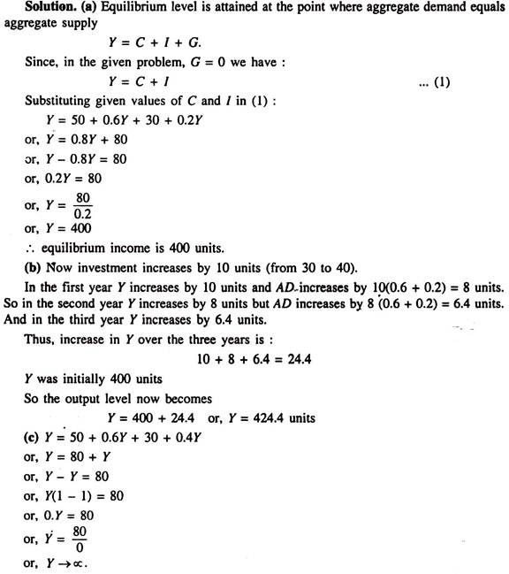
(a) Consider a simple Keynesian model where C = 50 + 0.6Y and I = 30 + 0.2 Y. The country is closed without government. Determine the equilibrium national income of the country.

(b) Suppose that in this country last year’s aggregate demand determines this year’s production. If autonomous investment rises from 30 to 40 then what will be the national income in three years’ time?

(c) If, starting from the situation described in (a), the investment function changes to I = 30 + 0.4K, what will happen to national income?

 

The consumption function for a simple economy is given by C = 310 + 0.7 Y_d

(a) Write an expression for saving in the economy.

(b) Express consumption in terms of Y when direct taxation is levied (i) as a lumpsum tax, T = 300, or (ii) as a proportional income tax, t = 0.4. Add these consumption functions to your diagram showing the consumption function without taxation and comment.

Solution

(a) Using the relationship S = Y_d– C we substitute the consumption function and obtain

5 = Y_d– (310 + 0.7 Y_d) = Y_d– 310 – 0.7 Y_d

Collecting terms gives the saving function

S = – 310 + 0.3 Y_d

With no direct taxation, Y_d = Y and the consumption and saving functions become

C = 310 + 0.7 Y

S = – 310 + 0.3 Y

(b) (i) With direct taxation, Y_d= Y – T. When T = 300, the consumption function becomes

C = 310 + 0.7 (Y – 300) or

C = 310 + 0.7 Y- 210 = 100 + 0.7 Y

A lumpsum tax shifts as consumption function down parallel to the original consumption function. (Students should check this point by drawing a suitable diagram.)

(ii) Using the relationship that with a proportional income tax Y_d = (1 – t) Y, since t = 0.4 we have Y_d = (1 – 0.4) Y = 0.6 Y. Substituting this in the consumption function gives

C = 310 + (0.7 x 0.6 Y) = 310 + 0.42 Y

Defects of the SKM:

The simple Keynesian model, presented in this chapter, is incomplete. It ignores money and interest rates and fails to explain the behaviour of prices and wages. Yet the model is useful in more “ways than one.

Firstly, the model clearly illustrates the role of aggregate demand in determining equilibrium income in a closed economy. No doubt aggregate demand plays a key role in determining income in the SKM. But it overstates the role of aggregate demand. This is why the autonomous expenditure multiplier is higher than in the IS-LM curve model (to be studied in Chapters 9 and 10).

In Keynes’ view, changes in autonomous expenditure, especially private investment demand, cause changes in equilibrium level of income. Changes in primary investment also induce changes in consumption spending. As a result, national income rises by a multiple of the initial increase in investment.

The increase in national income is equal to the primary investment (autonomous) plus a chain of secondary consumption spending. According to Keynes, the root cause of unemployment and depression is inadequate investment, and a consequent low level of aggregate demand.

The model also highlights the role of compensatory fiscal policy to stabilise the economy. Fiscal policy can be used to manage aggregate demand to restore equilibrium output which fluctuates due to unstable investment demand.

Here we have considered a simple closed economy. However, the model can be extended to cover an open economy.