The Keynes’ Theory of Demand for Money (With Diagram)

The Keynes’ Theory of Demand for Money!

Keynes treated money also as a store of value because it is an asset in which an individual can store his (her) wealth.

To Keynes an individual’s total wealth consisted of money and bonds.

Keynes used the term ‘bonds’ to refer to all risky assets other than money.

So money holding was the only alternative to holding bonds. And the only determinant of an individual’s portfolio choice was the interest rate on bonds.

This would affect an individual’s decision to divide his portfolio into money and bonds. To Keynes, it costs money to hold money and the rate of interest is the opportunity cost of holding money. At high rates of interest an individual loses a large sum by holding money or by not holding bonds.

Capital gain/loss:

Another factor affecting an individual’s portfolio choice was expected change in the rates of interest which would give rise to capital gain or loss. According to Keynes when the interest rate was high relative to its normal level people would expect it to fall in near future. A fall in the rate of interest would imply a Capital gain on bonds. According to Keynes at a high rate of interest there would be low demand for money as a store of value (wealth).

There are two reasons for this:

(i) At high rate of interest the opportunity cost of money holding (in terms of forgone interest) is high.

(ii) At a high rate of interest future capital gain on bonds is likely due to a fall in the rate of interest in future. It is because there is an inverse relation between the rate of interest and the price of old bonds. Thus if the present rate of interest is high, people will expect it to fall in near future, in which case they will expect to make capital gain.

Since the demand for money would fall at high rates of interest, and increase at low rates of interest, there is an inverse relation between the asset (speculative) demand for money and the rate of interest.

Keynes also considered transactions and precautionary demand for money whose primary determinant was income. Such demand would increase proportionately with increase in income.

So Keynes’ demand function for money can be expressed as

M_d = L(Y, i) … (3)

where Y is income and i is nominal interest rate and L stands for liquidity preference.

Policy Conclusions:

Thus, in Keynes’ view, the demand for money is a function of both income and interest rate, though in the classical theory, it was a function of income alone. This point is important in explaining the differences in policy conclusions between the classical and Keynesian models.

1. Determination of nominal income by the supply of money:

If the demand for money is exactly proportional to income, as in equations (1) and (2), then nominal income (PY) is completely determined by the supply of money. Since M= M_d = kPY, if k is assumed to remain fixed in equation (1) an increase in money supply (M) in equilibrium would result-in a proportional increase in PY. So we get

ΔM = kΔPY

or, 1/K ΔM = Δ PY … (4)

Thus equation (4) makes it abundantly clear that PY can change only when M changes, k remaining fixed. This means that changes in fiscal policy or autonomous changes in investment demand have no role in determining the equilibrium value of income. This is indeed the classical case of vertical LM curve, in which if M is fixed the level of income is automatically fixed. And any shift of the IS curve will only affect the rate of interest.

2. Role of fiscal policy change in income determination:

In Keynes’ money demand function, income is not proportional to the supply of money. This means that income changes can occur due to changes in fiscal policy and autonomous shifts in investment demand. In this case the LM curve will be upward sloping and any shift of the IS curve will change the equilibrium value of income. Of course, slopes of the IS and LM curves will determine the relative importance of monetary factors and other determinants of income (that shift the IS curve).

The Monetarists’ View:

The monetarists believe that the LM curve is quite steep, although not vertical. This largely, if not entirely, explains why money exerts a dominant influence on nominal income.

The Regressive Expectations Model:

According to Keynes the demand for money refers to the desire to hold money as an alternative to purchasing an income-earning asset like a bond. All theories of demand for money give a different answer to the basic question: If bonds earn interest and money does not why should a person hold money? The first theory to answer these questions known as the Keynesian theory of demand for money is based on a model called the regressive expectations model.

This essentially says that people hold money when they expect bond prices to fall, that is, interest rates to rise, and, thus, expect that they would incur a loss if they were to hold bonds. ‘Bonds’ here represent the whole range of risky assets that exist in reality. Since people’s estimates of whether the interest rate is likely to rise or fall — and by how much — vary widely, at any given interest rate there will be some people expecting it to rise and, thus, they would be holding money.

According to the regressive expectations model a bond holder has an expected return on the bond from two sources, the bond’s yield — the interest, payment he receives — and a potential capital gain — an increase in the price of the bond from the time he buys it to the time he sells it. The bond’s yield i is normally expressed as a percentage yield equal to Y divided by the face value of the bond. Thus

i = Y/P_b …(5)

Since the yield Y is fixed percentage of the bond’s face value, the market price of a bond is given by the ratio of yield to market rate:

P_b = Y/I …(6)

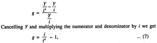
The expected percentage capital gain is the percentage increase in price from the purchase price P_b to the expected sale price P^e_b. From this we can derive the percentage capital gain, g = (P^e_b – P_b)/P_b. From equations (5) and (6), with a fixed Y on the bond, we can get an expected price P^e_b, corresponding to an expected interest rate, i_e = Y/P^e_b. Thus, in terms of expected and current interest rates, the capital gain can be expressed as

This is the expression for expected capital gain in terms of current and expected interest rates.

The total percentage return (earning) on a bond — denoted by e — is the sum of the market rate of interest at the time of purchase plus capital gains, e = i + g. Now if we substitute for g from equation (7), we get an expression for the total percentage return as the sum of interest yield and capital gains:

Now, with an expected return on bonds given by e, and with a zero return on money, the asset-holder can be expected to put his liquid wealth into bonds, if he expects the return e to be positive. If the return on bonds is expected to be negative, he will put all his liquid wealth into money.

In Keynes’ regressive expectations model, each person is assumed to have an expected interest rate i^e corresponding to some normal long-run average rate that is likely to prevail in the market. If actual rate rises above his long-run expectation, he expects them to fall, and vice versa.

Thus, his expectations are regressive. Here we assume that his expected long- run rate does not change much with changes in current market conditions.

The investor’s expected interest rate i^e, together with the actual market interest rate i, determines his expected percentage return e. On the basis of this we can compute the critical level of the market rate i_c, which would give him a net zero return on bonds, that is, the value of i that makes e = 0.

When actual i > i_c, we would expect him to hold all his liquid wealth in bonds. When i < i_c, he moves 100%, into money. To find this critical value, i_c, we set the total return shown in equation (8) equal to zero:

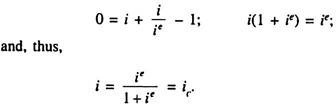
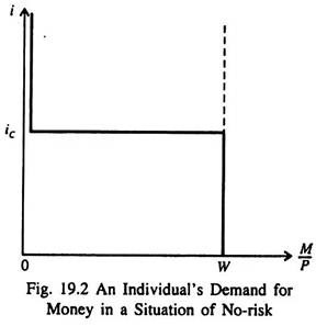
Here i_c, the critical market rate of interest that makes e = 0, is expressed as i^e/( 1 + i^e). This relationship between the individual’s demand for real balances and the interest rate is shown in Fig. 19.2. Here we show the demand for real balances on the horizontal axis.

It is the demand for real balances, M/P, that depends on the interest rate. Since we are implicitly holding the general price level con­stant, changes in real balances M/P correspond to changes in M.

In Fig. 19.2, if i exceeds i_c, the investor puts all his W into bonds, and his demand for money is zero. As i falls below i_c — so that expected capital losses on bonds exceed the interest yield and e becomes negative — the investor transfers his entire liquid wealth into money.

This give us a demand-for-money curve — for an individual — that looks like a step function. When i exactly equals e = 0 and the investor cannot choose between bonds and money. At any other value of i, the investor is either 100% in money or 100% in bonds.

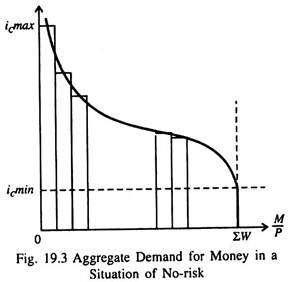
The individual demand curves of Fig. 19.2 can now be added up to get the total demand for money. Let us locate the individual with the highest critical interest rate, i_c^max in Fig. 19.3. As the interest rate falls below that i^max he shifts all of his liquid wealth into money.

As the interest rate falls, more individual i_cs are passed and more people shift from bonds to money. Ultimately, i will fall so much that no one will want to put his liquid wealth into bonds, and the demand for money will equal total liquid wealth, ∑W.

Thus, according to the average regressive expectations model as interest rates fall, the demand for money increases, and the demand curve is likely to be convex. Thus if the rate of interest continues to fall by the same percentage the demand for money will increase by increasing amounts.

The main problem with this view is that it suggests that individuals should, at any given time, hold all their liquid assets either in money or in bonds, but not some of each. So this is a all-or-nothing choice! This is obviously not true in reality.

There are two problems with this analysis. In the first, if the money market remained in equilibrium for a very long period, investors should gradually adjust their expected interest rates to cor­respond to the actual prevailing interest rate.

They would all tend to adopt eventu­ally the same critical interest rate with the passage of time. So the aggregate demand curve for money would look more and more like the flat curve of Fig. 19.2, instead of the negatively sloped demand curve with a variety of critical rates as shown in Fig. 19.3.

This prediction of the regressive ex­pectations model — that the elasticity of demand for money with respect to changes in the interest rate is increasing over time — is not supported by facts.

Secondly, if we assume that people actually do have a critical interest rate as shown in Fig. 19.3, then the model clearly implies that, in this two-asset world, investors hold either all bonds or all money, but not a mix of the two. The negative slope of the aggregate demand curve is due to the fact that investors differ in their opinion about the value of i^e, and, thus, in their critical rates i_c.

In fact, however, investors do not hold portfolios consisting of only one asset. As a general rule, portfolios contain a mixture of assets; they are diversified. This result — that people hold both money and bonds at the same time — has been explained by James Tobin.

Criticisms of Keynes’ Theory:

James Tobin found two main weaknesses of the Keynesian theory of the speculative demand for money:

(i) All-or-nothing choice:

In Keynes’ theory investors are assumed to hold all their wealth in bonds (other than the amount of money held for transaction purposes) as long as the rate of interest exceeded the ‘critical rate’ — a rate below which the expected capital loss on bonds outweighed the interest earnings on bonds.

If, on the contrary, the interest rate fell below the critical level, investors would hold no bonds, i.e., they would hold their entire wealth in money. So Keynes’ theory cannot explain why and how an individual investor diversifies his portfolio by holding both money and bonds as stores of wealth.

(ii) Changes in the normal rate of interest:

Keynes assumed that investors hold money as an asset so long as the interest rate is low. The reason is that they expect the interest rate to rise and return to ‘normal’ level. According to Keynes there exists a fixed or a slowly changing normal level for the interest rate, around which the actual rate of interest gravitates.

So the normal rate is taken as a benchmark against which to judge the possibility of interest rate changes which determine the amount of money held for speculative purposes.

According to Tobin the normal level itself keeps on changing over time — as has been shown by the experience of the 1950s. This explains why portfolio diversification takes place. An individual’s portfolio choice, i.e., his decision to diversify does not depend on Keynes’ restrictive assumption about investor expectations of a return of the interest rate to a normal level.

It is against this backdrop that we study Tobin’s portfolio theory of demand for money.

In short, Keynes’ followers such as James Tobin have not been satisfied with his theory of speculative demand for money which seeks to explain the inverse relationship between the interest rate and money demand. They have identified other reasons for the dependence of demand for money on the interest rate.

W. J. Baumol and Tobin have also extended Keynes’ analysis of the transactions demand for money. We may now discuss these two extensions of Keynes’ theory one by one.

On the other hand non-Keynesians — called monetarists — have refined and modified the classical quantity theory of money. This is another notable development in the area of monetary economics. Friedman’s analysis treats the demand for money in the same way as the demand for an ordinary commodity.

It can be viewed as a producer’s good; businesses hold cash balances to improve efficiency in their financial transactions and are willing to pay, in terms of forgone interest income, for this efficiency. Money can also be viewed as a consumer’s good; it yields utility to the consumer in terms of smoothing out timing differences between the expenditure and income streams and also in terms of reducing risk.