Linear and Non-Linear Consumption Function (With Diagram)

Linear and Non-Linear Consumption Function!

Linear Consumption Function:

There are two important concepts of propensity to consume, the one being average propensity to consume and the other marginal propensity to consume.

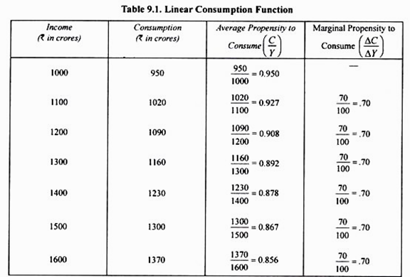
They should be carefully distinguished, for they are equal in some cases but different in others. Consider Table 9.1, where we have calculated the average and marginal propensity to consume in columns 3 and 4.

Consumption changes as income changes. Now, how much consumption changes in response to a given change in income depends upon the average and marginal propensity to consume. Thus, propensity to consume of a community can be known by the average and marginal propensity to consume.

Average Propensity to Consume:

Average propensity to consume is the ratio of the amount of consumption to total income. Therefore, average propensity to consume is calculated by dividing the amount of consumption by the total income. Thus,

APC = C/Y where Y

APC stands for average propensity to consume,

C for amount of consumption, and

Y for the level of income.

In Table 9.1 it will be seen that at the level of income Rs. 1000 crores, consumption expenditure is equal to Rs. 950 crores. Therefore, average propensity to consume is here equal to 950/100 = 0.95.

When the income rises to Rs. 1100 crores, consumption increases to Rs. 1020 crores. Therefore, the average propensity to consume will be 1020/1100= 0.927. In this schedule of consumption function, the average propensity to consume falls with the increase in income.

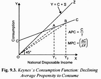
Keynesian consumption function CC is shown in Fig. 9.3. Average propensity to consume at a point on the consumption function curve can be obtained by measuring the slope of the ray from the origin to that point. For example, at income level OY₁ corresponding point on the consumption function curve is A.

Therefore, at OY₁income level, average propensity to consume (APC) is the slope of the ray OA. Similarly, at income level OY₁average propensity to consume is given by the slope of the ray OB. It will be observed from Fig. 9.3 that slope of OB is less than that of OA. Therefore, average propensity to consume at income level OY₂ is less than that at income level OY₁. In other words, average propensity to consume has declined with the increase in disposable income.

Non-Linear Consumption Function:

In the consumption function depicted in Fig. 9.3, though average propensity to consume(C/Y) declines, marginal propensity to consume which equals ∆C/∆Y remains constant since consumption function curve CC is a straight line and therefore its slope (∆C/∆Y)is constant.

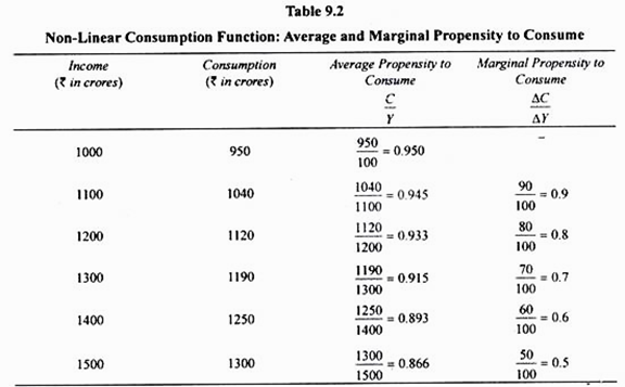
But it is not necessary that marginal propensity to consume should be the same at all levels of income. We have constructed in Table 9.2 another schedule of consumption function in which marginal propensity to consume declines with the increase in income.

 

It will be seen from Table 9.2 that when the level of income increases from Rs. 1000 crores to 1100 crores, consumption increases from 950 crores to 1040 crores, that, is by Rs. 90 crores. Therefore marginal propensity to consume is 0.9 and when income rises from 1400 crores to RS. 1500 crores, consumption increases by Rs. 50 crores from Rs. 1250 crores to 1300 crores.

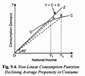
Therefore, marginal propensity to consume has declined to 0.5. When with the increase in income marginal propensity to consume declines, then the curve of consumption function is not a straight line but is convex from above as shown in Fig. 9.4.

In this case of non-linear consumption function average propensity to consume will also decline. At any point on the propensity to consume curve CC we can find out average propensity to consume by joining that point with the point of origin by a straight line whose slope will measure the average propensity to consume.

In Fig. 9.4, if we have to find out average propensity to consume at point A on the consumption function curve CC, we connect point A with the origin by a straight line. Now, the slope of the line OA i.e., AY₁\OY₁ will measure the average propensity to consume. Similarly, at point B of the given consumption function CC, the average propensity to consume will be given by the slope of the line OB which is equal to BY₂/OY₂ A glance at the Figure 9.4 Will show that the slope of the line OB is smaller than the slope of the line OA. Therefore, average propensity to consume at point B or at income level OY₂ is less than that at point A or income level OA ₁.

Marginal Propensity to Consume:

The concept of marginal propensity to consume is very important, because from it we can know how much part of the increment in income is consumed and how much saved. Marginal propensity to consume is the ratio of change in consumption to the change in income. Thus:

MPC = ∆Y/∆Y

where, MPC stands for marginal propensity to consume,

∆C for change in consumption, and

∆T for change in income.

Marginal propensity to consume needs to be carefully distinguished from average propensity to consume. Whereas average propensity to consume is the ratio of total consumption to total income,

i.e., C/Y, the marginal propensity to consume is the ratio of change in consumption to the change in income, i.e. ∆C/∆Y.

The concept of marginal propensity to consume can be easily understood with the aid of Table 9.2 in column 4 of which we have calculated the marginal propensity to consume at various levels of income. In this schedule when income rises from Rs. 1000 crores to Rs. 1100 crores, the consumption increases from Rs. 950 crores to Rs. 1040 crores. Here the increment in income is t 100 crores but the increment in consumption is Rs. 90 crores. Therefore, marginal propensity to consume which is ∆C/∆Y is here equal to 90/100 or 0.9.

Similarly, when national income rises to Rs. 1200 crores and as a result consumption increases from Rs. 1040 crores to Rs. 1120 crores, the marginal propensity to 80 consume is now equal to 80/100 or 0.8. In Table 9.2, it will be seen that marginal propensity to consume declines as the income rises. It is worth noting that when with the increase in income average propensity to consume declines, marginal propensity to consume is less than average propensity to consume. This is in accordance with the usual relationship between the average and marginal quantities. This is evident from Table 9.2.

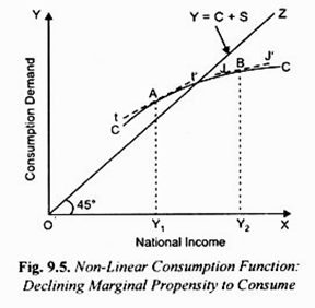
Marginal propensity to consume can be estimated by drawing the tangent at a point on the consumption function. Consider Fig. 9.5 where curve CC depicting the consumption function has been drawn. Marginal propensity to consume at point A on this will be equal to the slope of the tangent tt’ drawn at this point. Similarly, marginal propensity to consume at point B on it is given by the slope of the tangent JJ drawn at this point. It will be seen that slope of the tangent JJ is less than the slope of the tangent tt’.

Therefore, marginal propensity to consume at point B on the consumption function CC in Fig. 9.5 is smaller than the marginal propensity to consume at point A on this consumption function. Thus, marginal propensity to consume is declining with the increases in income in the non-linear consumption function curve CC in Fig. 9.5.

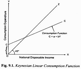
Thus when marginal propensity to consume declines with the increase in income, consumption function is non-linear whose slope declines as income rises. Non-linear consumption function is shown in Fig. 9.5 where the slope of the propensity to consume curve CC declines as income increases. In Fig. 9.1 and Fig. 9.3 propensity to consume curve is a straight line i.e., the slope of the consumption function curve remains constant. Therefore, marginal propensity to consume which is given by the slope of the consumption function curve remains constant in Fig. 9.1 and 9.3.

It is worth noting that marginal propensity to consume is neither zero nor equal to one. It has been found by empirical studies that marginal propensity to consume varies between zero and unity. If the marginal propensity to consume was zero, then the whole of the increment in income would have been saved and the consumption function curve would have a horizontal shape.

On the other hand, if the marginal propensity to consume was equal to unity, then the whole of the increment in income would be consumed and in that case consumption function curve would have coincided with 45° line.