Top 4 Types of Hypothesis in Consumption (With Diagram)

The following points highlight the top four types of Hypothesis in Consumption. The types of Hypothesis are: 1. The Post-Keynesian Developments 2. The Relative Income Hypothesis 3. The Life-Cycle Hypothesis 4. The Permanent Income Hypothesis.

Hypothesis Type # 1. The Post-Keynesian Developments:

Data collected and examined in the post-Second World War period (1945-) confirmed the Keynesian consumption function.

Time series data collected over long periods showed that the relation between income and consumption was different from what cross-section data revealed.

In the short run, there was a non-proportional relation between income and consumption. But in the long run the relation was proportional. By constructing new aggregate data on consumption and income from 1869 and examining the same, Simon Kuznets discovered that the ratio of consumption to income was fairly stable from decade to decade, despite large increases in income over the period he studied.

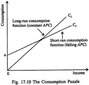
This contradicted Keynes’ conjecture that the average propensity to consume would fall with increases in income. Kuznets’ findings indicated that the APC is fairly constant over long periods of time. This fact presented a puzzle which is illustrated in Fig. 17.10.

Studies of cross-section (household) data and short time series confirmed the Keynesian hypothesis — the relationship between consumption and income, as indicated by the consumption function C_s in Fig. 17.10.

But studies of long time series found that APC did not vary systematically with income, as is shown by the long-run consumption func­tion C_L. The short-run consumption function has a falling APC, whereas the long-run consumption function has a constant APC.

Subsequent research on consumption at­tempted to explain how these two consump­tion functions could be consistent with each other.

Various attempts have been made to rec­oncile these conflicting evidences. In this context mention has to be made of James Duesenberry (who developed the relative income hypothesis), Ando, Brumberg and Modigliani (who developed the life cycle hypoth­esis of saving behaviour) and Milton Friedman who developed the permanent income hypothesis of consumption behaviour.

All these economists proposed explanations of these seemingly contradictory findings. These hypotheses may now be discussed one by one.

Hypothesis Type # 2. The Relative Income Hypothesis:

In 1949, James Duesenberry presented the relative income hypothesis. According to this hypothesis, saving (consumption) depends on relative income. The saving function is expressed as S_t =f(Y_t/ Y_p), where Y_t / Y_p is the ratio of current income to some previous peak income. This is called relative income. Thus current consumption or saving is not a function-of current income but relative income.

Duensenberry pointed out that during depression when income falls consumption does not fall much. People try to protect their living standards either by reducing their past savings
(or accumulated wealth) or by borrowing.

However as the economy gradually moves initially into the recovery and then in to the prosperity phase of the business cycle consumption does not rise even if income increases. People use a portion of their income either to restore the old saving rate or to repay their old debt.

Thus we see that there is a lack of symmetry in people’s consumption behaviour. People find it more difficult to reduce their consumption level than to raise it. This asymmetrical behaviour of consumers is known as the ratchet effect.

Thus if we observe a consumer’s short-run behaviour we find a non-proportional relation between income and consumption. Thus MPC is less than APC in the short run, as Keynes’s absolute income hypothesis has postulated. But if we study a consumer’s behaviour in the long run, i.e., over the entire business cycle we find a proportional relation between income and consumption. This means that in the long run MPC = APC.

Hypothesis Type # 3. The Life-Cycle Hypothesis:

In the late 1950s and early 1960s Franco Modigliani and his co-workers Albert Ando and Richard Brumberg related consumption expenditure to demography. Modigliani, in particular, emphasised that income varies systematically over peoples’ lives and that saving allows consumers to move income from early years of earning (when income is high) to later years after retirement when income is low.

This interpretation of household consumption behaviour forms the basis of his life-cycle hypothesis.

The life cycle hypothesis (henceforth LCH) represents an attempt to deal with the way in which consumers dispose off their income over time. In this hypothesis wealth is assigned a crucial role in consumption decision. Wealth includes not only property (houses, stocks, bonds, savings accounts, etc.) but also the value of future earnings.

Thus consumers visualise themselves as having a stock of initial wealth, a flow of income generated by that wealth over their lifetime and a target (which may be zero) as their end-of-life wealth. Consumption decisions are made with the whole series of financial flows in mind.

Thus, changes in wealth as reflected by unexpected changes in flow of earnings or unexpected movements in asset prices would have an impact on consumers’ spending decisions because they would enhance future earnings from property, labour or both. The theory has empirically testable implications for the relation between saving and age of a person as also for the role of wealth in influencing aggregate consumer spending.

The Hypothesis:

The main reason that an individual’s income varies is retirement. Since most people do not want their current living standard (as measured by consumption) to fall after retirement they save a portion of their income every year (over their entire service period). This motive for saving has an important implication for an individual’s consumption behaviour.

Suppose a representative consumer expects to live another T years, has wealth of W, and expects to earn income Y per year until he (she) retires R years from now. What should be the optimal level of consumption of the individual if he wishes to maintain a smooth level of consumption over his entire life?

The consumer’s lifetime endowments consist of initial wealth W and lifetime earnings RY. If we assume that the consumer divides his total wealth W + RY equally among the T years and wishes to consume smoothly over his lifetime then his annual consumption will be:

C = (W + RY)/T … (5)

This person’s consumption function can now be expressed as

C = (1/T)W + (R/T)Y

If all individuals plan their consumption in the same way then the aggregate consumption function is a replica of our representative consumer’s consumption function. To be more specific, aggregate consumption depends on both wealth and income. That is, the aggregate consumption function is

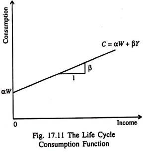
C = αW + βY …(6)

where the parameter α is the MPC out of wealth, and the parameter β is the MPC out of income.

Implications:

Fig. 17.11 shows the relationship between consumption and income in terms of the life cycle hypothesis. For any initial level of wealth w, the consumption function looks like the Keynesian function.

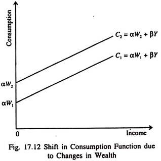
But the intercept αW which shows what would happen to consump­tion if income ever fell to zero, is not a constant, as is the term a in the Keynesian consumption function. Instead the intercept αW depends on the level of wealth. If W increases; the consumption line will shift up­ward parallely.

So one main prediction of the LCH is that consumption depends on wealth as well as income, as is shown by the intercept of the consumption function.

Solving the consumption puzzle:

The LCH can solve the consumption puzzle in a simple way.

According to this hypothesis, the APC is:

C/Y = α(W/Y) + β … (7)

Since wealth does not vary proportionately with income from person to person or from year to year, cross-section data (which show inter-individual differences in income and consumption over short periods) reveal that high income corresponds to a low APC. But in the long run, wealth and income grow together, resulting in a constant W/Y and a constant APC (as time-series show).

If wealth remains constant as in the short run the life cycle consumption function looks like the Keynesian consumption function, consumption function shifts upward as shown in Fig. 17.12. This prevents the APC from falling as income increases.

This means that the short-run consumption income relation (which takes wealth as constant) will not continue to hold in the long run when wealth increases. This is how the life cycle hypothesis (LCH) solves the consumption puzzle posed by Kuznets’ studies.

Other Predictions:

Another important prediction made by the LCH is that saving varies over a person’s lifetime. The LCH helps to link consumption and savings with the demo­graphic considerations, especially with the age distribution of the population.

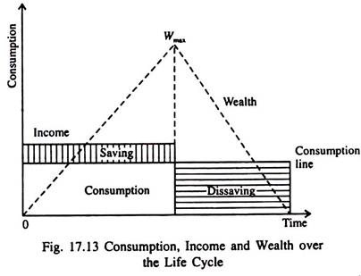
The MPC out of life-time income changes with age. If a person has no wealth at the beginning of his service life, then he will accumulate wealth over his working years and then run down his wealth after his retirement. Fig. 17.13 shows the consumer’s income, consumption and wealth over his adult life.

If a consumer smoothest consumption over his life (as indicated by the horizontal consumption line), he will save and accumulate wealth during his working years and then dissave and run down his wealth after retirement. In other words, since people want to smooth consumption over their lives, the young — who are working — save, while the old — who have retired — dissave.

In the long run the consumption-income ratio is very stable, but in the short run it fluctuates. The life cycle approach explains this by pointing out that people seek to maintain a smooth profile of consumption even if their lifetime income flow is uneven, and thus emphasises the role of wealth in the consumption function.

Theory and Evidence: Do Old People Dissave?

Some recent findings present a genuine problem for the LCH. Old people are found not to dissave as much as the hypothesis predicts. This means that the elderly do not reduce their wealth as fast as one would expect, if they were trying to smooth their consumption over their remaining years of life.

Two reasons explain why the old people do not dissave as much as the LCH predicts:

(i) Precautionary saving:

The old people are very much concerned about unpredictable expenses. So there is some precautionary motive for saving which originates from uncertainty. This uncertainty arises from the fact that old people often live longer than they expect. So they have to save more than what an average span of retirement would warrant.

Moreover uncertainty arises due to the fact that the medical expenses of old people increase faster than their age. So some sort of Malthusian spectre is found to be operating in this case. While an old person’s age increases at an arithmetical progression his medical expenses increase in geometrical progression due to accelerated depreciation of human body and the stronger possibility of illness.

The old people are likely to respond to this uncertainty by saving more in order to be able to overcome these contingencies.

Of course, there is an offsetting consideration here. Due to the spread of health and medical insurance in recent years old people can protect themselves against uncertainties about medical expenses at a low cost (i.e., just by paying a small premium).

Now-a-days various insurance plans are offered by both government and private agencies (such as Medisave, Mediclaim, Medicare, etc.). Of course, the premium rate increases with age. As a result the old people are required to increase their saving rate to fulfill their contractual obligations.

However, to protect against uncertainty regarding lifespan, old people can buy annuities from insurance companies. For a fixed fee, annuities offer a stream of income over the entire life span of the recipient.

(ii) Leaving bequests:

Old people do not dissave because they want to leave bequests to their children. The reason is that they care about them. But altruism is not really the reason that parents leave bequests. Parents often use the implicit threat of disinheritance to induce a desirable pattern of behaviour so that children and grandchildren take more care of them or be more attentive.

Thus LCH cannot fully explain consumption behaviour in the long run. No doubt providing for retirement is an important motive for saving, but other motives, such as precautionary saving and bequest, are no less important in determining people’s saving behaviour.

Another explanation, which differs in details but entirely shares the spirit of the life cycle approach is the permanent income hypothesis of consumption. The hypothesis, which is the brainchild of Milton Friedman, argues that people gear their consumption behaviour to their permanent or long term consumption opportunities, not to their current level of income.

An individual does not plan consumption within a period solely on the basis of income within the period; rather, consumption is planned in relation to income over a longer period. It is to this hypothesis that we turn now. We may now turn to Friedman’s permanent income hypothesis, which suggests an alternative explanation of long-run income-consumption relationship.

Hypothesis Type # 4. The Permanent Income Hypothesis:

Milton Friedman’s permanent income hypothesis (henceforth PIH) presented in 1957, comple­ments Modigliani’s LCH. Both the hypotheses argue that consumption should not depend on current income alone.

But there is a difference of insight between the two hypotheses while the LCH emphasises that income follows a regular pattern over a person’s lifetime, the PIH emphasises that people experience random and temporary changes in their incomes from year to year.

The PIH, Friedman himself claims, ‘seems potentially more fruitful and in some measure more general” than the relative income hypothesis or the life-cycle hypothesis.

The idea of consumption spending that is geared to long-term average or permanent income is essentially the same as the life cycle theory. It raises two further questions. The first concerns the precise relationship between current consumption and permanent income. The second question is how to make the concept of present income operational, that is how to measure it.

The Basic Hypothesis:

According to Friedman the total measured income of an individual Y_m has two compo­nents : permanent income Y_p and transitory income Y_t. That is, Y_m – Y_p + Y_t.

Permanent income is that part of income which people expect to earn over their working life. Transitory income is that part of income which people do not expect to persist. In other words, while permanent income is average income, transitory income is the random deviation from that average.

Different forms of income have different degrees of persistence. While adequate investment in human capital (expenditure on training and education) provides a permanently higher income, good weather provides only transitorily higher income.

The PIH states that current consumption is not dependent solely on current disposable income but also on whether or not that income is expected to be permanent or transitory. The PIH argues that both income and consumption are split into two parts — permanent and transitory.

A person’s permanent income consists of such things as his long term earnings from employment (wages and salaries), retirement pensions and income derived from possessions of capital assets (interest and dividends).

The amount of a person’s permanent income will determine his permanent consumption plan, e.g., the size and quality of house he buys and, thus, his long term expenditure on mortgage repayments, etc.

Transitory income consists of short-term (temporary) overtime payments, bonuses and windfall gains from lotteries or stock appreciation and inheritances. Negative transitory income consists of short-term reduction in income arising from temporary unemployment and illness.

Transitory consumption such as additional holidays, clothes, etc. will depend upon his entire income. Long term consumption may also be related to changes in a person’s wealth, in particular the value of house over time. The economic significance of the PIH is that the short run level of consumption will be higher or lower than that indicated by the level of current disposable income.

According to Friedman consumption depends primarily on permanent income, because consumers use saving and borrowing to smooth consumption in response to transitory changes in income. The reason is that consumers spend their permanent income, but they save rather than spend most of their transitory income.

Since permanent income should be related to long run average income, this feature of the consumption function is clearly in line with the observed long run constancy of the consumption income ratio.

Let Y represent a consumer unit’s measured income for some time period, say, a year. This, according to Friedman, is the sum of two components : a permanent component (Y_p) and a transitory component (Y_t), or

Y = Y_P + Y_t …(8)

The permanent component reflects the effect of those factors that the unit regards as determining its capital value or wealth the non-human wealth it owns, the personal attributes of the earners in the unit, such as their training, ability, personality, the attributes of the economic activity of the earners, such as the occupation followed, the location of the economic activity, and so on.

The transitory component is to be interpreted as reflecting all ‘other’ factors, factors that are likely to be treated by the unit affected as ‘accident’ or ‘chance’ occurrences, for example, illness, a bad guess about when to buy or sell, windfall or chance gains from race or lotteries and so on. Permanent income is some sort of average.

Transitory income is a random variable. The difference between the two depends on how long the income persists. In other words, the distinction between the two is based on the degree of persistence. For example education gives an individual permanent income but luck — such as good weather — gives a farmer transitory income.

It may also be noted that permanent income cannot be zero or negative but transitory income can be.

Suppose a daily wage earner falls sick for a day or two and may not earn anything. So his transitory income is zero. Similarly if an individual sales a share in the stock exchange at a loss his transitory income is negative. Finally permanent income shows a steady trend but transitory income shows wide fluctuation(s).

Similarly, let C represent a consumer unit’s expenditures for some time period. It is also the sum of a permanent component (C_p) and a transitory component (C_t), so that

C = C_p + C_t … (9)

Some factors producing transitory components of consumption are: unusual sickness, a specifically favourable opportunity to purchase and the like. Permanent consumption is assumed to be the flow of utility services consumed by a group over a specific period.

The permanent income hypothesis is given by three simple equations (8), (9) and (10):

Y = Y_p + Y_t …(8)

C – C_p + C_t …(9)

C_p = kY_p, where k = f (r, W, u) …(10)

Here equation (6) defines a relation between permanent income and permanent consump­tion. Friedman specifies that the ratio between them is independent of the size of permanent income, but does depend on other variables in particular: (i) the rate of interest (r) or sets of rates of interest at which the consumer unit can borrow or lend; (ii) the relative importance of property and non-property income, symbolised by the ratio of non-human wealth to income (W) (iii) the factors symbolised by the random variable u determining the consumer unit’s tastes and preference for consumption versus additions to wealth. Equations (8) and (9) define the connection between the permanent components and the measured magnitudes.

Friedman assumes that the transistory components of income and consumption are uncorrelated with one another and with the corresponding permanent components, or

P_ytyp = P_ctcp = P_ytct = 0 …(11)

where p stands for the correlation coefficient between the variables designated by the subscripts. The assumption that the third component in equation (11) — between the transitory components of income and consumption — is zero is indeed a strong assumption.

As Friedman says:

“The common notion that savings,…, are a ‘residue’ speaks strongly for the plausibility of the assumption. For this notion implies that consumption is determined by rather long-run considerations, so that any transitory changes in income lead primarily to additions to assets or to the use of previously accumulated balances rather than to corresponding changes in consumption.”

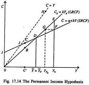
In Fig. 17.14 we consider the con­sumer units with a particular measured income, say which is above the mean measured income for the group as a whole — Y’. Given zero correlation be­tween permanent and transitory compo­nents of income, the average permanent income of those units is less than Y₀; that is, the average transitory component is positive.

The average consumption of units with a measured income Y₀ is, therefore, equal to their average perma­nent consumption. In Friedman’s hy­pothesis this is k times their average permanent income.

If Y₀ were not only the measured income of these units but also their permanent income, their mean consumption would be Y₀ or Y₀E. Since their mean permanent income is less than their measured income (i.e., the transitory component of income is positive), their average consumption, Y₀F, is less than Y₀E.

By the same logic, for consumer units with an income equal to the mean of the group as a whole, or Y, the average transitory component of income as well as of consumption is zero, so the ordinate of the regression line is equal to the ordinate of the line 0E which gives the relation between Y_p and C_p.

For units with an income below the mean, the average transitory component of income is negative, so average measured consumption (CC”) is greater than the ordinate of 0E (BC’). The regression line (C = a + bY), therefore, intersects 0E at D, is above it to the left of D, and below it to the right of D.

If k is less than unity, permanent consumption is always less than permanent income. But measured consumption is not necessarily less than measured income. The line OH is a 45° line along which C = Y.

The vertical distance between this line and IF is average measured savings. Point J is called the ‘break-even’ point at which average measured savings are zero. To the left of J, average measured savings are negative, to the right, positive; as measured income increases so does the ratio of average measured savings to measured income.

Friedman’s hypothesis thus yields a relation between measured consumption and measured income that reproduces the broadest features of the corresponding regressions that have been computed from observed data. The point is that consumption expenditures seem to be proportional to disposable income in the long run.

In the short run, on the other hand, the consumption-income ratio fluctuates considerably. In sum, current consumption is related to some long-run measure of income (e.g., permanent income) while short-run fluctuations in income tend primarily to affect the level of saving.

Estimating Permanent Income:

Dornbusch and Fischer have defined permanent income as “the steady rate of consumption a person could maintain for the rest of his or her life, given the present level of wealth and income earned now and in the future.”

One might estimate permanent income as being equal to last year’s income plus some fraction of the change in income from last year to this year:

where α is a fraction and Y_t-1, is last year’s income. Equation (8) suggests that permanent income is a weighted average of current and past income.

If Y_t = Y_t-1 that is, if this year’s income is equal to last year’s, then permanent income is equal to the income earned this year and last year. This ensures that an individual who had always earned the same income would expect to earn that income in the future.

Another point to note is that if income rises this year compared with last year, then permanent income rises by less than current income. The reason is easy to find out the individual does not know whether the rise in income this year is permanent.

Without knowing whether the increase in income will be maintained or not, the individual does not immediately increase the expected or permanent income measure by the full amount of the actual or current increase in income.

Predictions:

1. Specification error:

According to PIH, consumption depends on present income. But the Keynesian absolute income hypothesis relates consumption to current income. Friedman solves the consumption puzzle by suggesting that the Keynesian consumption function uses the wrong variable.

2. Behaviour of APC:

In Friedman’s model, APC is expressed as C_p/Y_m = kY_p. This means that APC depends on the ratio of permanent income to current income. As N.G. Mankiw has put it: “When current income temporarily rises above permanent income, the average propensity to consume temporarily falls; when current income temporarily falls below permanent income, the average propensity to consume rises.”

3. Consumption levels:

Friedman reasoned on the basis of cross-section data, that households with high permanent income have proportionately higher consumption. It there­fore follows by deduction that households with transitory income do not consume much.

As Mankiw has interpreted the PIH:

“If all variation in current income came from the permanent component, the APC would be the same in all households but some of the variation in income comes from the transitory components, and households with high transitory income do not have higher consumption. Therefore, high income households have an average, lower average propensities to consume.”

4. Constant APC in the long-run:

Friedman argued that year-to-year fluctuations in income are dominated by transitory income. This means that years of high income should be years of low average propensities to consume. But over long periods of time — say, from one decade to another — the variation in income is largely due to the permanent component. Hence in long time-series, a constancy of APC is to be observed, as found by Kuznets.

5. Rational expectations:

Nobel Laureate R. Lucas has suggested that if consumers obey the PIW and have rational expectations, then only unexpected policy changes influence consumption. These policy changes make their effect felt when they change expectations.

A substantial part of the consumption function relates to Friedman’s PIH which treats consumption decision as based on a longer run concept of income and receipts during some arbitrary accounting period such as a year but in the Friedman model consumption (defined as the using up of goods and services, not their acquisition) is being analysed, not consumer expenditure.

Thus the PIH has little to say directly about the causes of cyclical variation in consumer spending unless permanent income is itself affected by cyclical change—in which case the desired stock of durable goods will change and net investment or disinvestment in such goods will occur.

Beyond PIH:

The PIH provides appealing explanations of many important features of consumption. For example it explains why a temporary taxed card has a much smaller effect than a permanent one.

Yet, there are certain important features of consumption that appear inconsistent with the PIH. For example both macroeconomic and microeconomic evidences suggest that consump­tion responds to predictable changes in income. Indeed the PIH fails to explain some central features of consumption behaviour.

One of Friedman’s predictions is that there should be no relation between the expected growth of an individual’s income over his lifetime and the expected growth of his consumption; consumption growth is determined by the real interest rate and the discount rate, not by the time pattern of income.

Recent statistical studies suggest that his prediction of PIH is incorrect. For example, individuals in countries where income growth is high, normally have high rates of consump­tion growth over their lifetime and individuals in slowly growing countries usually have low rates of consumption growth.

Similarly, typical lifetime consumption patterns of individuals in different occupations try to match typical lifetime income patterns in those occupations. For example, managers and professionals normally have fastly growing incomes until their middle age, then their income remains fairly steady. So their consumption profiles follow a similar pattern.

More generally households having little wealth depend much on their income, so their current income has a larger role in determining their consumption. Yet, these households use whatever small savings they have to prevent their consumption from falling in the event of sharp falls in income.

They also use the savings if there is any emergency spending need thus most households exhibit buffer-stock saving behaviour. These failings of PIH have motivated the search for alternatives to the theory.

The PIH can be saved by suggesting an explanation of the fact that most households have little wealth as has been postulated by Friedman. The truth is that welfare programmes rather than buffer-stock savings provide insurance against very low level of consumption. This is one way of saving the PIH.