Intertemporal Choice and Budget Constraint (With Diagram) | Consumption Function

Let us make an in-depth study of the Intertemporal Choice and Budget Constraint. After reading this article you will learn about: 1. Intertemporal Choice 2. The Intertemporal Budget Constraint 3. Deriving the Budget Constraint 4. Interpretation 5. Time Indifference Curves.

Intertemporal Choice:

According to Keynes’ absolute income hypothesis current consumption depends only on current income.

But this assumption is not always true. In reality while taking consumption and saving decisions people consider both the present and the future.

The more the people consume in the current period (today or the current year) and the Jess they save, the less they will be able to consume in the next period (tomorrow or next year).

So there is always a choice (trade-off) between current consumption and future consumption. So in making consumption decisions households have to take into consideration their expected future income as also the consumption of goods and services they are likely to be able to afford.

Irving Fisher developed a model to analyse how rational, forward-looking consumers make consumption choices over a period of time.

Fisher’s model of intertemporal choice illustrates at least three things:

(1) the budget constraints faced by consumers,

(2) their preferences between current and future consumption, and

(3) how these two conjointly determine households’ decision regarding optimal consumption and saving over an extended period of time. Modern economist have gone one step ahead of this and have included borrowing constraints also while analysing consumption choice over time.

The Intertemporal Budget Constraint:

Rational individuals always prefer to increase the quantity or quality of the goods and services they consume. However, most people cannot consume as much as they like due to limited income. In other words, people face a budget constraint, which sets a limit on how much they can spend.

Since consumption decisions are taken over a period of time, consumers face intertemporal budget constraint, which shows how much income is available for consumption now and in the future. This constraint reflects a consumer’s decision on how much to consume today and how much to save for the future.

For the sake of simplicity let us assume that our representative consumer lives for two periods — period 1 is his youth and period 2 is his old age. His income and consumption in the two periods are Y₁, and C₁ and Y₂ and C₂, respectively. Here we ignore price level changes or express all variables in real terms (after making adjustment for price inflation).

Since the consumer can borrow and save, consumption in any period need not necessarily be equal to his current income: Y₁, ≠ C₁, and Y₂ ≠ C₂.

Consumption in two periods is constrained by income in two periods.

In the first period saving (5) is the difference between income and consumption:

S = Y₁ – C₁ … (1)

In the second period consumption equals the accumulated saving (which includes the interest earned on that saving), plus second-period income:

C₂ = (1 + r)S + Y₂ … (2)

where r is the real interest rate (i.e., nominal interest adjusted for inflation). Since we do not consider the third period, the consumer is not required to save in the second period.

The variable S may represent either saving or borrowing. Equations (1) and (2) hold in both cases. If C₁ < Y₁, S > 0. If C₁ > Y₁, S < 0, i.e., the consumer is borrowing. We assume, for the sake of simplicity, that interest rate for saving (and lending) and borrowing are the same.

Deriving the Budget Constraint:

We can now derive the consumer’s budget constraint by combining equations (1) and (2). If we substitute the first equation for S into the second equation we get

C₂ = (1 + r) (Y₁ – C₁) + Y₂ … (3)

or, (1 + r) C₁ + C₂ = (1 + r)Y₁ + Y₂

[by bringing (1 + r) C, from the r.h.s. to the l.h.s.]

Finally by dividing both sides of equation (3) by 1 + r we get:

C₁ + C₂ / 1 + r = Y₁ + Y₂ / 1 + r… (4)

Since this equation relates consumption in two periods to income in both the periods it expresses the consumers’ intertemporal budget constraint.

Interpretation:

If r = 0, equation (4) shows that C₁ + C₂ = Y₁ + Y₂, i.e., total consumption in the two periods equals total income in the two periods. But in the real world in which r > 0, C₂ and r₂ are to be discounted by a factor 1 + r. Since it is possible to earn interest by saving (i.e., by sacrificing current consumption) this discount factor has to be used while making intertemporal choice between consumption and saving.

Since r > 0, Y₂ (= Rs.100, say) < Y₁ (= Rs.100). This means that since a consumer earns interest on saving, future income is less than the same amount of current income. In a like manner, since future consumption expenditure is made from accumulated saving (which includes earned interest), the cost of future consumption is less than that of current consumption. The discount factor 1/(1 + r) measures how much period 1 consumption has to be sacrificed in order to consume 1 unit in period 2.

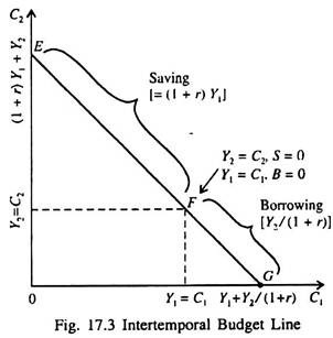
In Fig. 17.3 the line EFJG is the consumer’s intertemporal budget con­straint. It shows the alternative combina­tions of period 1 and period 2 consumption the consumer can choose. If the consumer is at point F, he consumes his entire income in both the periods (Y₁ = C₁ and Y₂ = C₂, S = 0, B = 0). At point E, C₁ = 0 and Y₁ = S.

Therefore C₂ = (1 + r)Y₁ + Y₂. Thus if he chooses points between E and F, he consumes less than his income in period 1 and saves the rest for period 2.

At point G, C₂ = 0. This means that the consumer borrows the maximum possible amount against Y₂. This means that C₁ is Y₁ + Y₂/(1 + r). Thus if he chooses any point between F and G, he consumes more than his income in period 1 and borrows to make-up the difference. Various other points on the budget line EFG are attainable points.

Time Indifference Curves:

Time indifference curves may now ‘ be drawn to represent the consumer’s preference regarding consumption in period 1 and period 2. A time indiffer­ence curve is a locus of points showing alternative combinations of C₁ and C₂ that yield the same satisfaction to the consumer.

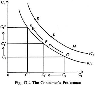
Fig. 17.4 shows two indifference curves of the consumer — IC₁ and 1C₂. We can think of any number of such indifference curves. The consumer is indifferent among points E, F and G, because they all lie on the same indif­ference curve. If the consumer moves from point G to F, C₁ falls to C’₁ So C₂ must increase to C’₂ to keep him equally satisfied.

Otherwise, he cannot be indifferent between the two points G and F showing two different combinations of C₁ and C₂. If C₁ is reduced again from F to E, he requires a greater amount of extra C₂ as compensation.

The slope of an indifference curve at any point indicates how much C₂ the consumer requires as compensation for sacrificing C₁ by 1 unit. So the slope is the marginal rate of substitution between C₁ and C₂. It is the desired rate of intertemporal substitution, i.e., the rate at which the consumer is willing to substitute C₂ for C₁ while staying on the same indifference curve.

Since C₁ and C₂ are not perfect substitutes of each other, i.e., the pain involved in sacrificing C₁ and the gain made by increasing the level of C₂ are not the same at all the points on the indifference curve, it is not a straight line. As a result, the MRS depends on the levels of consumption in the two periods.

When C₁ is high and C₂ is low, as at point G, the MRS is low. This means that the consumer needs only a little extra C₂ to sacrifice every extra unit of C₁. When C₁ is low and C₂ is high, as at point E, the MRS is high the consumer needs much extra C₂ in order to forego 1 unit of C₁.

Since more satisfaction is always preferred to less, the consumer prefers higher indif­ference curves to lower ones. [The reason for this is explained in the standard theory of consumer demand which is studied extensively in microeconomic theory]. In Fig. 17.4 he prefers points K, L, M, etc. on indifference curve IC₂ to the points E, F, G, etc. on indifference curve IC₁.

Indifference curves can be used to rank any combinations of C₁ and C₂.